Supervised and Unsupervised Learning in Machine Learning

Supervised learning

Core concepts and principles

Definition and Analogy (Teacher-Guided Learning)

• Supervised machine learning is a fundamental paradigm where a model is systematically trained on labeled data.
• This implies that every input data point within the training set is explicitly paired with its correct, desired output.
• This learning process is often conceptualized through the analogy of a teacher guiding a student.
• The model, acting as the student, learns by continuously comparing its predictions against the actual, correct answers provided within the training data.
• Through this iterative comparison, the model adjusts its internal parameters to progressively minimize errors and enhance its predictive accuracy over time.

For instance, in a task involving handwritten digit recognition, the model is exposed to numerous images of digits, each meticulously labeled with its corresponding numerical value (e.g., an image of '5' explicitly tagged as '5').

This labeled exposure enables the model to discern the characteristic features associated with each digit.

Similarly, a dataset comprising various fruit images would have each image precisely tagged with its correct fruit name, such as "Apple" or "Banana," allowing the model to learn to differentiate between them.

How Supervised Learning Works (Training, Testing, Prediction)

• The operational workflow of supervised learning typically unfolds in two distinct yet interconnected phases: the training phase and the testing phase.
• During the training phase, the algorithm is provided with a comprehensive training dataset.
• This dataset is rich with both input data, often referred to as 'features,' and their corresponding output data, known as 'labels' or 'target variables'.
• The algorithm meticulously processes this labeled information, deciphering the intricate relationships and underlying patterns that connect the input features to their respective output labels.
• This learning involves a continuous adjustment of the model's internal parameters, a process aimed at minimizing the discrepancy between its generated predictions and the true labels present in the training data.
• The iterative refinement ensures the model progressively becomes more adept at recognizing the patterns it is being taught.

Following the training phase, the model's predictive prowess is rigorously assessed during the testing phase.

Here, the trained model is presented with a new, entirely unseen test set.

This crucial evaluation step gauges the model's generalization capability,its capacity to accurately predict outcomes on data it has not previously encountered.

A well-trained model is expected to perform robustly on this unseen data, demonstrating its learned understanding rather than mere memorization of the training examples.

The comprehensive process of developing a supervised model involves several critical steps:

Meticulous data collection and preprocessing

1. The strategic division of data into training (e.g., 80%)
2. The test (e.g., 20%) sets
3. The actual training of the model
4. A thorough evaluation of its performance using various quantitative metrics
5. Hyperparameter tuning to optimize its settings for peak performance.

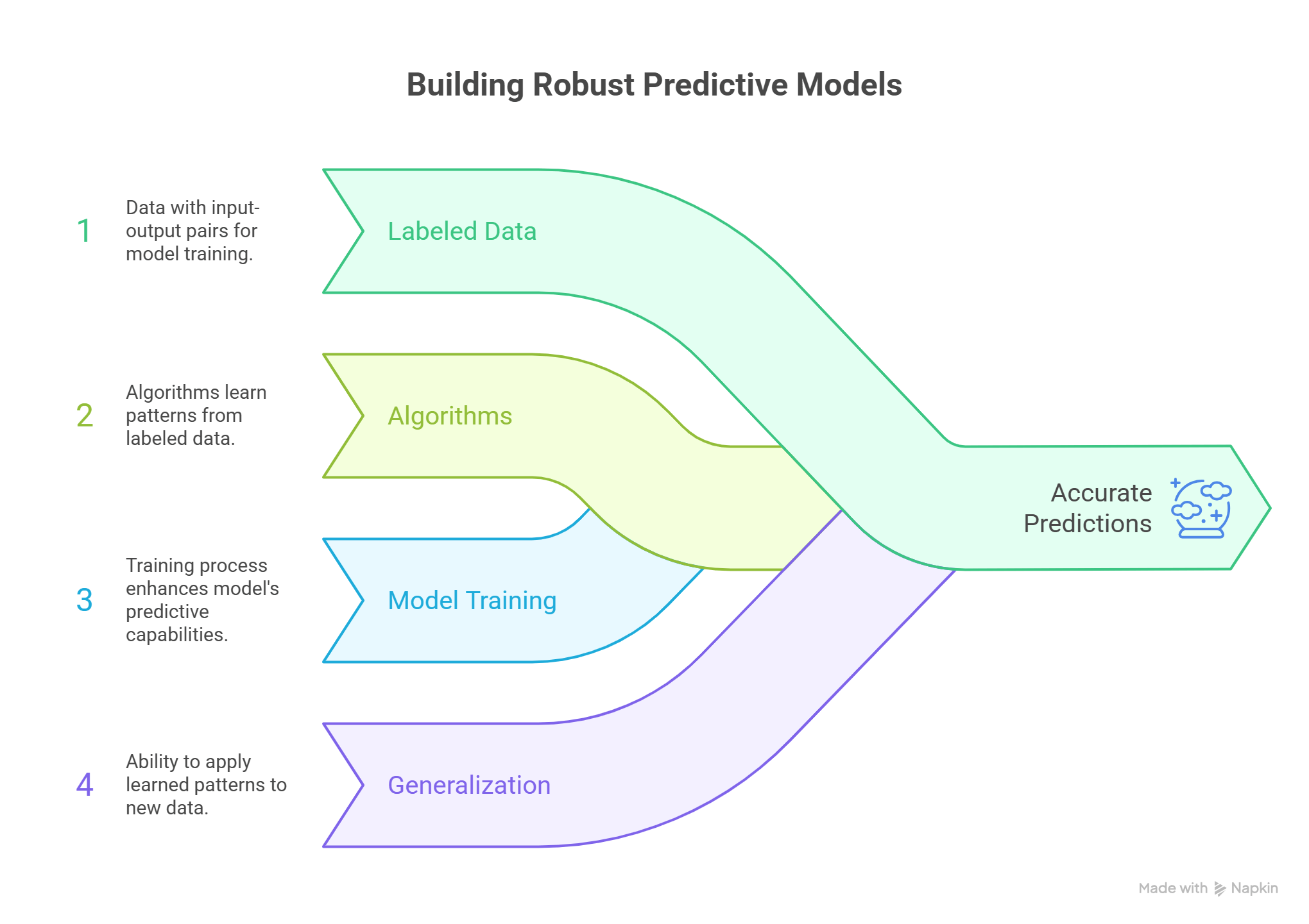
Key Characteristics and Goals

• The overarching objective of supervised learning is to achieve robust generalization to unseen data and to produce highly accurate predictions.
• By learning from a multitude of labeled examples, the model develops the ability to make precise forecasts or classifications on new, previously unobserved data.
• A notable characteristic is that with an increase in the volume of training data and continued iterative training, these models consistently enhance their accuracy, leading to improved performance and more reliable predictions in practical applications.
• Supervised learning models are inherently designed to predict specific outcomes or to classify data into predefined categories.
• Consequently, they are exceptionally well-suited for problem domains where the desired output is clearly defined, measurable, and where a discernible "correct" answer exists for each input.
• The entire supervised learning workflow, from data preparation to model evaluation, is fundamentally structured around this pedagogical approach.
• The labeled data serves as the "correct answers" in the curriculum, the iterative learning process is analogous to a student's repeated practice, and the evaluation on unseen data is akin to a final examination assessing the student's ability to solve new problems independently.

This deep connection ensures that the model's learning is always directed towards a specific, measurable goal.

Types of Supervised Learning Problems

Supervised learning is broadly applied to two primary categories of problems, distinguished by the intrinsic nature of the output variable that the model is tasked with predicting.

Classification: Categorical Predictions

• Classification tasks involve predicting a discrete class label or a specific category for a given input.
• In these scenarios, the output is a categorical variable, meaning it falls into one of a finite set of predefined classes.
• Common examples include binary classifications such as "spam vs. non-spam emails," "yes vs. no," or "malignant vs. benign" in medical diagnoses.
• It also extends to multi-class classification, like identifying different file types or categorizing images.

• For instance, an email spam filter operates by analyzing various features of an incoming email, such as keywords, sender information, and message structure, to classify it as either spam or legitimate.
• Similarly, image classification systems categorize visual data into predefined classes, such as distinguishing between images of cats and dogs based on learned visual features.

Regression: Continuous Value Predictions

• Regression tasks, in contrast to classification, involve predicting a continuous value or a quantifiable quantity.
• Here, the output is a numerical variable that can take any value within a given range, rather than being confined to discrete categories.

• Illustrative examples include predicting real estate prices, forecasting stock market trends, estimating daily temperatures, or determining a person's salary based on their years of work experience.
• For example, a regression model designed to forecast house prices would consider a multitude of features, such as square footage, the number of bedrooms, and geographical location, to output a continuous numerical price estimate.

• This fundamental dichotomy in the nature of the predicted output discrete categories versus continuous values is a foundational concept in supervised learning.
• It directly influences the selection of appropriate algorithms, the choice of evaluation metrics, and ultimately, defines the specific type of problem that supervised learning can effectively address.

The clarity of this distinction enables the development of specialized and highly effective solutions for a wide range of predictive challenges.

Prominent Supervised Learning Algorithms

A diverse array of algorithms falls under the supervised learning paradigm, each possessing unique characteristics that make it suitable for different types of problems and data structures.

Linear Regression

• Linear Regression is a fundamental supervised machine learning algorithm primarily employed for regression tasks.

• Its core purpose is to predict continuous numerical values by modeling a linear relationship between one or more input features (independent variables) and a target variable (dependent variable).

• The operational principle of Linear Regression revolves around finding the "best-fit" straight line in a two-dimensional space, or a hyperplane in higher-dimensional spaces, that minimizes the discrepancy between the observed data points and the values predicted by the model.

• This minimization is typically achieved through the Ordinary Least Squares (OLS) method, which calculates the sum of the squared differences (residuals) between the actual and predicted values, and then seeks to minimize this sum.

• For simple linear regression, involving a single independent variable, the relationship is expressed by the equation ŷ = β₀ + β₁x, where ŷ represents the predicted value of the dependent variable, x is the input (independent variable), β₁ (or m) is the slope of the line indicating the change in ŷ for a unit change in x, and β₀ (or b) is the intercept, representing the value of ŷ when x is zero.

• This model can be extended to ŷ = β₀ + β₁x₁ + β₂x₂ +... + βnxn for multiple independent variables, known as multiple linear regression.
• Linear Regression operates under several key assumptions, including linearity (a straight-line relationship between variables), independence of errors (predictions should not influence each other), and homoscedasticity (constant variance of errors across all input values).

• A classic example is predicting house prices based on features like square footage, or forecasting a student's exam score based on the number of hours they studied.

Logistic Regression

• Despite its nomenclature, Logistic Regression is not a regression algorithm in the traditional sense of predicting continuous values; rather, it is a statistical algorithm predominantly utilized for binary classification tasks.

• Its primary function is to predict outcomes that fall into one of two discrete classes, such as "yes/no," "spam/not spam," or "true/false".
• The model can also be adapted for multiclass classification problems through strategies like the "one-vs-all" approach.

• Instead of fitting a straight line to data points, Logistic Regression employs an "S"-shaped curve known as the logistic function or sigmoid function.
• This function is crucial because it maps any real-valued input into an output probability ranging strictly between 0 and 1, making it ideal for modeling probabilities of class membership.

• The mathematical representation of the sigmoid function is f(z) = 1 / (1 + e^-z), where z is a linear combination of the input features and their corresponding weights (z = β₀ + β₁x₁ +... + βnxn).
• The output y' from the sigmoid function is interpreted as the probability of the instance belonging to the positive class.

• A predefined threshold value (commonly 0.5) is then applied to these probabilities to assign the final class label: probabilities above the threshold are classified as one class, and those below as the other.
• The optimization of Logistic Regression models typically involves minimizing a logarithmic loss function, often referred to as cross-entropy loss or log loss.

• This loss function is convex, which facilitates the use of optimization algorithms like gradient descent to efficiently find the optimal model parameters.
• Examples of its application include predicting whether an email is spam or assessing an individual's susceptibility to a particular disease based on medical parameters.

Support Vector Machines (SVM)

• Support Vector Machines (SVM) constitute a powerful supervised learning algorithm capable of addressing both classification and regression tasks, though they are particularly renowned for their efficacy in binary classification problems.

• The fundamental principle behind SVM is to identify the "best boundary," or hyperplane, that optimally separates different classes within the dataset.
• The "best" hyperplane is not merely one that separates the classes, but specifically one that maximizes the margin the maximal distance between the hyperplane and the closest data points from each class.

• These closest data points are critically important and are known as support vectors, as they directly influence the position and orientation of the optimal hyperplane.

• A significant strength of SVM lies in its ability to handle data that is not linearly separable, meaning data points that cannot be perfectly divided by a straight line or a simple hyperplane in their original feature space.
• For such scenarios, SVM employs a sophisticated technique called the "kernel trick".

• A kernel function implicitly maps the data into a higher-dimensional feature space where it becomes linearly separable, without the computationally intensive process of explicitly computing the coordinates in that higher space.

• Commonly utilized kernel functions include the Linear kernel for linearly separable data, the Polynomial kernel, and the Radial Basis Function (RBF) kernel, which is highly versatile for complex, non-linear relationships.

• SVM models can be configured with either a "hard margin," which demands perfect separation with no misclassifications, or a "soft margin," which tolerates a certain degree of misclassification or margin violations to enhance generalization, especially when dealing with noisy data or outliers.
• Misclassifications in soft margin SVMs are penalized, often using a "hinge loss" function.
• Practical applications include classifying cancer cells as 'malignant' or 'benign' based on their features or filtering spam emails.

Decision Trees

• Decision Trees are non-parametric supervised learning algorithms that are remarkably versatile, applicable to both classification and regression tasks.
• A key advantage of Decision Trees is their inherent interpretability; their structure closely mimics human decision-making processes, making the logic behind their predictions relatively easy to understand and visualize.

• The fundamental structure of a Decision Tree is hierarchical and resembles a flowchart.
• It comprises a root node (representing the entire dataset), internal nodes (also known as decision nodes, where decisions based on specific features are made), branches (representing the outcomes of these decisions), and leaf nodes (or terminal nodes, which represent the final decision or prediction).

• The operational mechanism of a Decision Tree is based on a "divide and conquer" strategy.
• The algorithm recursively partitions the dataset into increasingly homogeneous subsets. At each internal node, the data is split based on the value of a chosen feature.

The selection of the optimal feature for splitting at each node is governed by splitting criteria, which quantitatively measure the "purity" or "impurity" of the resulting subsets.

Two prominent splitting criteria are:

Entropy

• This metric quantifies the amount of uncertainty or randomness within a set of data.
• A lower entropy value indicates a higher degree of purity, meaning the subset is more homogeneous with respect to the target variable.
• Entropy is typically employed in algorithms such as ID3 and C4.

Gini Impurity

• This measure calculates the probability that a randomly selected element from a set would be incorrectly classified if it were randomly labeled according to the distribution of labels within that subset.
• A lower Gini impurity signifies greater purity.
• Gini impurity is a hallmark of the CART (Classification and Regression Trees) algorithm.

To mitigate overfitting a common problem where a model performs exceptionally well on training data but poorly on new, unseen data a technique called pruning is often applied.

Pruning involves systematically removing unnecessary branches from the tree that contribute little to generalization, typically those splitting on features of low importance.

An illustrative example of a Decision Tree's application is deciding whether to add a particular movie to a watch list based on criteria such as its genre, IMDB rating, and whether it has been watched previously.

The choice of supervised algorithm often involves a practical trade-off between interpretability and predictive complexity.

Algorithms like Linear Regression and Decision Trees are highly valued for their simplicity and the ease with which their decision-making processes can be understood.

This transparency is crucial in domains where understanding why a prediction was made (e.g., medical diagnoses, financial risk assessments) is as vital as the prediction itself.

In contrast, algorithms such as Support Vector Machines, particularly when employing kernel tricks to map data into higher dimensions, can become highly complex and less directly interpretable, even if they offer superior predictive accuracy for certain non-linear problems.

Logistic Regression occupies an intermediate position, providing probabilistic outputs that offer some level of transparency. This spectrum of interpretability highlights the growing importance of "explainable AI" (XAI) in practical machine learning deployments.

Furthermore, a deep understanding of the mathematical principles underpinning each algorithm is critical, as these foundations directly dictate their behavior, strengths, and inherent limitations. For instance, Linear Regression's reliance on minimizing squared errors leads to its sensitivity to outliers but also its simplicity.

Logistic Regression's use of the sigmoid function for probability estimation and cross-entropy loss explains its effectiveness in binary classification but also its challenges with highly non-linear data without feature engineering.

SVM's margin maximization objective, coupled with the kernel trick, explains its robustness and ability to handle complex data. Decision Trees' splitting criteria, such as entropy or Gini impurity, directly determine how they partition data and their susceptibility to overfitting without pruning.

This underscores that effective model selection, tuning, and troubleshooting in machine learning require not just practical application skills but also a strong theoretical grounding in the mathematical underpinnings of these algorithms.

Advantages of Supervised Learning

Supervised learning, despite its inherent requirements, offers several compelling advantages that make it a cornerstone of modern machine learning applications:

High Accuracy and Reliability

• Models trained on meticulously labeled data can achieve exceptionally high accuracy in predicting outcomes on new, unseen data.
• This precision is critical in high-stakes domains such as medical diagnostics, where accurate predictions can directly impact patient outcomes, and in financial forecasting, where even small errors can have significant monetary repercussions.
• The explicit feedback from labels allows for continuous refinement and optimization.

Clear Goals and Measurable Performance

• The presence of a defined, labeled output variable provides a clear target for the model's learning process.
• This clarity facilitates straightforward evaluation using a suite of well-established metrics. For classification tasks, metrics like accuracy, precision, and recall offer quantitative measures of performance, while for regression tasks, Mean Squared Error (MSE) and R-squared are commonly employed.
• This clear framework allows practitioners to objectively assess how well their model performs against known outcomes.

Enhanced Algorithm Efficiency with Feature Learning

• By learning from labeled datasets, supervised models are not only trained to predict but also to discern and prioritize the most crucial features within the input data that are relevant for accurate predictions.
• This inherent capability for feature learning optimizes the overall learning process, reducing complexity and improving the model's performance over time, which is particularly valuable in dynamic environments like automated trading or real-time anomaly detection.

Robust Performance in Controlled Environments

• Supervised learning models demonstrate robust and predictable performance in environments where the problem is well-defined, and the relationship between input data and output is stable and clearly understood.
• Their ability to learn explicit mappings makes them highly effective in such structured settings.

Wide Range of Mature Algorithms

• The field of supervised learning boasts a rich and mature ecosystem of algorithms.
• Established and well-understood algorithms such as Linear Regression, Logistic Regression, Support Vector Machines (SVM), Decision Trees, Random Forest, K-Nearest Neighbors (KNN), and Naive Bayes are readily available and suitable for a diverse array of tasks.
• This breadth of tools allows practitioners to select the most appropriate algorithm for a given problem, often with extensive community support and documentation.

Disadvantages of Supervised Learning

Despite its numerous advantages, supervised learning is not without its limitations, primarily stemming from its fundamental reliance on labeled data:

Dependency on Labeled Data

• The most significant drawback of supervised learning is its absolute reliance on large, high-quality, and meticulously labeled datasets for training.
• The process of creating such datasets is often an arduous undertaking, demanding substantial investments in time, financial resources, and human effort.
• This labeling process frequently requires domain expertise, making it a costly and labor-intensive bottleneck.
• In many real-world scenarios, particularly where data is generated continuously or involves subjective interpretations, obtaining precise and comprehensive labels can be impractical or even infeasible, severely restricting the applicability of supervised learning.
• This "cost of knowledge" the human effort and expense involved in annotating data is a primary constraint for supervised learning.
• This economic and logistical bottleneck has directly spurred innovation in other machine learning paradigms, such such as semi-supervised and self-supervised learning, which aim to mitigate this dependency by leveraging abundant unlabeled data.

Limited Generalization to Unseen/Complex Data

• While generally capable of high accuracy, supervised models can sometimes struggle with generalization, particularly when confronted with data that significantly deviates from the patterns observed in their training set.
• This issue is often manifested as overfitting, where the model learns the training data too precisely, including its noise and idiosyncrasies, leading to poor performance on new, unseen data.
• Furthermore, these models may struggle with highly complex or unstructured problems that involve abstract ideas or nuanced patterns not explicitly represented in their labeled training examples.

Vulnerability to Noisy or Biased Data

• The quality of predictions from a supervised learning model is directly contingent upon the quality of its input data and labels.
• If the training data contains noise (errors, inconsistencies) or inherent biases, the model will inevitably learn and perpetuate these flaws.
• This susceptibility can lead to skewed results, inaccurate predictions, and potentially discriminatory outcomes, highlighting the critical importance of rigorous data curation and bias detection in the labeling process.

Computational Intensity

• Training supervised learning models, especially deep learning architectures with vast amounts of labeled data, often demands significant computational resources.
• This can translate into substantial processing power, memory, and time, posing a challenge for organizations with limited infrastructure or tight deadlines.

Real-World Applications of Supervised Learning

Supervised learning forms the technological backbone for a vast and diverse array of real-world applications across nearly every industry, demonstrating its utility in solving problems that require precise, verifiable predictions.

Spam Filtering

• One of the most ubiquitous applications, supervised learning is extensively used in email systems to accurately classify incoming emails as either legitimate or spam.
• Models are trained on large datasets of emails meticulously labeled as "spam" or "non-spam," learning to identify characteristic patterns, keywords, and sender behaviors associated with unwanted messages.

Fraud Detection

• Financial institutions heavily rely on supervised learning algorithms to combat fraudulent activities. By analyzing historical transaction data labeled as either legitimate or fraudulent, models learn to identify suspicious patterns and anomalies, enabling real-time flagging of potentially fraudulent transactions in banking, e-commerce, and insurance.

Image Classification and Object Recognition

• Supervised learning powers systems capable of categorizing images into predefined classes and identifying specific objects or individuals within them.
• This includes applications like automatically tagging friends in social media photos, facial recognition for security or mobile device unlocking, and object detection in autonomous vehicles to recognize pedestrians and obstacles.
• In the medical domain, supervised learning is crucial for analyzing medical images (X-rays, MRIs) to detect diseases like cancer with high accuracy, often surpassing human capabilities in early detection.

Medical Diagnosis and Prognosis

• Supervised learning is indispensable in healthcare for assessing the likelihood of various diseases and predicting patient outcomes.
• Models are trained on patient features, historical medical records, and diagnostic results to assist in tasks like classifying cancer cells as 'malignant' or 'benign,' or predicting the risk of heart disease.

Natural Language Processing (NLP)

• Supervised learning is fundamental to numerous NLP tasks, enabling machines to understand, interpret, and generate human language.

Sentiment Analysis

• Determines the emotional tone or sentiment expressed in text data, crucial for customer feedback analysis and social media monitoring.

Machine Translation

• Facilitates the automatic translation of text from one language to another.

Named Entity Recognition (NER)

• Identifies and categorizes key entities such as names of persons, organizations, and locations within text.

Text Classification

• Categorizes text documents into predefined topics or genres.

Speech Recognition

• Powers voice assistants like Apple's Siri and Amazon's Alexa, converting spoken commands into text and interpreting user intent.

Predictive Analytics and Forecasting

• Supervised learning is widely used for forecasting future trends and outcomes across various sectors.

Stock Price Prediction

• Models analyze historical market data, trading volumes, and economic indicators to predict future stock prices or trends.

House Price Prediction

• Forecasts real estate values based on features like size, location, number of bedrooms, and local market conditions.

Risk Assessment

• Financial services utilize supervised models to assess credit risk, predict loan defaults, or evaluate insurance claims, helping to minimize financial exposure.

Recommendation Systems

• While often complemented by unsupervised methods, supervised learning can contribute to recommendation engines by learning from past user behavior (e.g., viewing history, purchase history) to predict user preferences and suggest relevant products, movies, or content.

The pervasive nature of supervised learning in these applications, particularly in high-stakes domains like fraud detection, medical diagnosis, and financial forecasting, underscores its critical role.

In these areas, accuracy and reliability are paramount, and the consequences of error can be severe.

This indicates that despite the challenges associated with acquiring and labeling data, the investment is often justified by the need for precise, verifiable predictions with clear "right" or "wrong" answers.

Supervised learning's maturity and trustworthiness in these established domains make it the preferred method when high-confidence outcomes are required.

Unsupervised learning

Core concepts and principles

Definition and Analogy (Self-Discovery)

• Unsupervised learning represents a distinct paradigm within machine learning, characterized by its ability to learn from data without human supervision or explicit guidance.

• In contrast to supervised learning, unsupervised models are presented with unlabeled data raw information devoid of predefined categories or target outputs.

• The algorithms are then tasked with autonomously discovering inherent patterns, structures, and insights within this data.
• This process is often likened to an explorer navigating an unfamiliar island without a map.

• The explorer observes the terrain, notes recurring features like paths leading to beaches or the boundaries of forests, and gradually constructs an understanding of the island's underlying structure through self-exploration and pattern recognition.

• The algorithm, similarly, must discern how to group or organize the data solely based on its intrinsic characteristics.

How Unsupervised Learning Works (Pattern Identification)

• Unsupervised learning algorithms operate through self-learning mechanisms, meticulously analyzing unlabeled data to identify underlying patterns, relationships, and structural regularities on their own.

• Since the data lacks any predefined categories or outcomes, the algorithm is compelled to discover these patterns intrinsically, without any external "teacher" providing correct answers.

• This task can be inherently challenging due to the absence of ground truth for validation, yet it can be immensely rewarding.
• The process has the potential to reveal profound insights into the data that would not be apparent or discoverable from a pre-labeled dataset.

• For instance, an unsupervised algorithm might analyze a large dataset of weather observations and autonomously group data points by temperature ranges or similar atmospheric conditions, effectively identifying "hot days" or "cold days" without ever being explicitly told what constitutes these categories.

• This capacity for autonomous pattern identification makes unsupervised learning a powerful tool for exploratory analysis.

Key Characteristics and Goals

• The primary objective of unsupervised learning is to extract meaningful insights from large volumes of new data by comprehending its underlying structure and identifying previously undetected patterns and relationships.

• This approach excels at exploratory data analysis, serving as a powerful tool for understanding how data points naturally group together or for reducing complex datasets into simpler, more manageable forms without compromising essential patterns.

• A significant characteristic that distinguishes unsupervised learning is its independence from labeled data.
• This eliminates the often time-consuming and expensive manual labeling process, making it considerably easier and quicker to initiate work with large, raw datasets.

• The core aim is not to predict a specific outcome, but rather to uncover the inherent organization of the data, allowing the machine learning system itself to determine what aspects of the dataset are distinct, interesting, or indicative of underlying structures.

• This positions unsupervised learning as a valuable tool for hypothesis generation and understanding data's inherent structure, rather than solely for prediction.
• It is particularly beneficial in scientific discovery and exploring new phenomena where predefined categories or outcomes are unknown or difficult to ascertain.

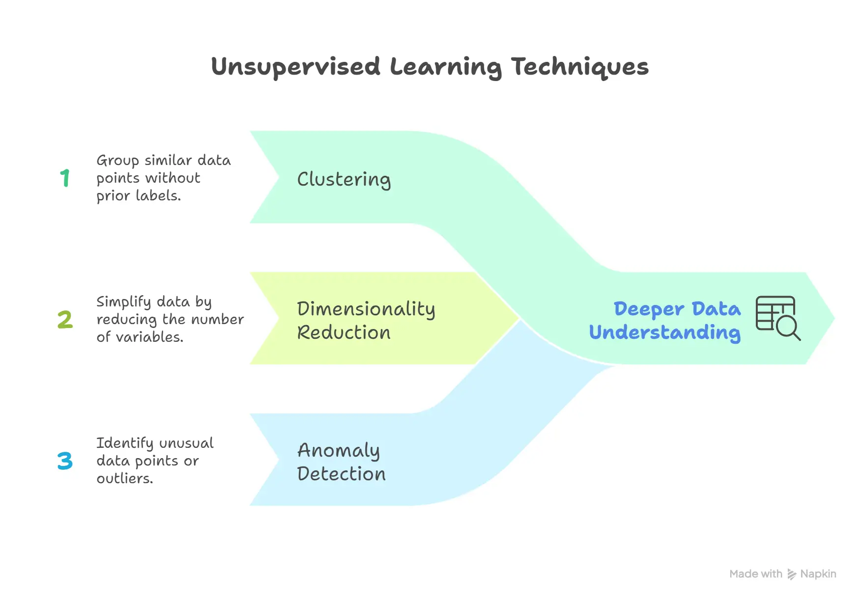
Types of Unsupervised Learning Tasks

Unsupervised learning models are predominantly utilized for three main categories of tasks, each designed to extract different types of information from unlabeled data:

Clustering: Grouping Similar Data

Clustering is a fundamental data mining technique that involves grouping unlabeled data points into coherent "clusters" based on their inherent similarities or differences.

The primary objective of clustering is to identify natural groupings and underlying patterns within the data without any prior knowledge of the data's meaning or predefined categories.

Various types of clustering algorithms exist to address different data structures and analytical needs:

Exclusive ("Hard") Clustering

In this approach, each data point is assigned to precisely one cluster, with no overlap. K-means clustering is a prominent example of exclusive clustering.

Overlapping ("Soft") Clustering

This allows a single data point to belong to two or more clusters simultaneously, often with varying degrees of membership or probability. Fuzzy C-means is an example of soft clustering.

Hierarchical Clustering

This method constructs a nested sequence of clusters, often visualized as a tree-like structure called a dendrogram.

It can be performed in two ways:

1. Agglomerative (bottom-up), starting with individual data points as clusters and iteratively merging the closest pairs,
2. Divisive (top-down), beginning with all data points in one cluster and recursively splitting them.

Probabilistic Clustering

• Data points are assigned to clusters based on the probability of belonging to each cluster, rather than strict similarity thresholds.
• A common application of clustering is in marketing, where it is used to group customers based on their purchase frequency, spending habits, or browsing behavior, enabling the creation of distinct customer segments like "Budget Shoppers" or "Frequent Buyers" for personalized marketing strategies.

Association Rule Learning: Finding Relationships

• Association rule learning is a technique focused on discovering frequent "if-then" patterns or associations within datasets.
• These rules reveal correlations and co-occurrences among data objects, highlighting relationships that might not be immediately obvious.

• The core idea is to identify rules such as "people who buy X often also buy Y".
• This method is extensively applied in market basket analysis, where it helps retailers understand customer purchasing habits, and in the development of recommendation engines.
• For instance, if analysis reveals that customers who purchase milk frequently also buy bread, eggs, or butter, a grocery store could leverage this information to optimize product placement or create bundled offers.

Dimensionality Reduction: Simplifying Data

• Dimensionality reduction is a crucial unsupervised learning technique applied when datasets contain an excessively high number of features or dimensions.

• The primary goal is to reduce the number of input variables to a more manageable size while diligently preserving the essential structure and integrity of the original data.

• This technique is invaluable for several reasons: it helps eliminate redundant information, significantly improves computational efficiency by reducing the processing load, and makes high-dimensional data much easier to visualize and analyze.

• For example, a dataset containing 100 features describing students (such as height, weight, grades, etc.) could be reduced to just two or three key features (e.g., height and grades) for simpler visualization or more efficient downstream analysis, without losing the most critical information.

• This process highlights that unsupervised learning, particularly dimensionality reduction, often functions as a critical preprocessing step.
• By simplifying complex data, it acts as an enabler for other machine learning tasks, including potentially supervised ones, making otherwise intractable datasets amenable to analysis and modeling.

Prominent unsupervised learning algorithms

Several algorithms are widely employed for unsupervised learning tasks, each offering distinct methodologies for uncovering patterns in unlabeled data.

K-Means Clustering

K-Means Clustering is a highly popular and widely adopted unsupervised machine learning algorithm designed to group unlabeled datasets into a predefined number of K distinct clusters, based on the inherent similarity of data points within each cluster.

The algorithm operates through an iterative refinement process:

1. Specify K: The process begins with the user explicitly defining the desired number of clusters, K.

2. Initialize Centroids: K initial "means" or cluster centroids are randomly generated or selected from within the data domain.

3. Assign to Clusters: Each data point in the dataset is then assigned to the closest centroid. The most common metric for determining "closest" is Euclidean distance, which quantifies the similarity between data points and centroids. This assignment step forms the initial clusters.

4. Update Centroids: Once all points are assigned, the centroids are re-calculated. Each new centroid becomes the average position (mean) of all data points currently assigned to its respective cluster.

5. Iterate: Steps 3 and 4 are repeated iteratively. The algorithm continues to re-assign data points and update centroids until the positions of the centroids no longer change significantly, or until the assignments of data points to clusters stabilize, indicating convergence.

The objective of K-Means is to minimize the within-cluster sum of squares (WCSS), which is the sum of the squared Euclidean distances between each data point and the centroid of its assigned cluster.

While K-Means is guaranteed to converge to a local optimum, it is important to note that it is not guaranteed to find the global optimum, meaning the best possible clustering solution. The initial placement of centroids can influence the final clustering outcome, and running the algorithm multiple times with different initializations can help mitigate this.

A practical application involves an online store using K-Means to group customers based on their purchase frequency and spending habits, thereby creating distinct customer segments for highly personalized marketing campaigns.

The iterative refinement loop in K-Means, where points are assigned and centroids are updated, exemplifies how unsupervised models learn by maximizing internal consistency rather than minimizing external errors.

This iterative nature also implies that the final solution can be sensitive to initial conditions, a characteristic common to many optimization-based unsupervised algorithms.

Hierarchical Clustering

• Hierarchical clustering is another prominent clustering algorithm that constructs a nested sequence of clusters, which is visually represented as a tree-like structure known as a dendrogram.
• This dendrogram provides a comprehensive view of how clusters are formed and merged (or split) at different levels of similarity.
• There are two primary types of hierarchical clustering:

Agglomerative (Bottom-Up)

• This is the most common approach. It begins by treating each individual data point as its own separate cluster.
• Subsequently, it iteratively merges the closest pairs of clusters based on a measure of similarity (or dissimilarity) between them.
• This merging process continues until all data points are consolidated into a single, large cluster. Various "linkage methods" define how the similarity between two clusters is measured, including Ward's linkage, Average linkage, Complete (maximum) linkage, and Single (minimum) linkage.

Divisive (Top-Down)

• This approach is the inverse of agglomerative clustering. It starts with all data points grouped into a single, large cluster.
• It then recursively divides this cluster into smaller, more distinct clusters based on differences between data points, continuing until each data point forms its own individual cluster.

• Hierarchical clustering is often used for tasks like grouping similar documents or images based on their content, or for genetic and species grouping in biological research, where understanding the relationships and nested structures is important.

Association Rule Learning (e.g., Apriori Algorithm)

• Association rule learning is a powerful unsupervised technique designed to uncover strong relationships or "rules" between items within large datasets, with widespread application in market basket analysis.
• The goal is to identify patterns such as "if a customer buys item X, they are also likely to buy item Y."
• The Apriori Algorithm stands as a classic and foundational algorithm in this domain.
• It systematically identifies frequent itemsets (combinations of items that frequently appear together in transactions) and subsequently generates association rules from these itemsets.
• A key efficiency of the Apriori algorithm stems from the "Apriori property": if an itemset is infrequent (does not meet a minimum frequency threshold), then all its supersets (any larger itemset containing it) will also be infrequent.

This property allows the algorithm to prune the search space significantly, improving computational efficiency.

The strength and significance of the discovered association rules are quantified using three key metrics:

1. Support

• This metric measures how frequently an itemset appears in the entire dataset relative to the total number of transactions.
• It indicates the overall popularity or prevalence of an item or combination of items.
• For example, Support({Bread}) = (Number of transactions containing Bread) / (Total number of transactions).

2. Confidence

• Confidence assesses the conditional likelihood that item Y is purchased given that item X has been purchased. It is essentially the conditional probability P(Y|X).
• For example, Confidence({Bread -> Butter}) = (Number of transactions containing Bread and Butter) / (Number of transactions containing Bread). It indicates the reliability of the rule.

3. Lift

• Lift quantifies the strength of the association between X and Y by comparing their co-occurrence to what would be expected if they were statistically independent. Lift(X -> Y) = Confidence(X -> Y) / Support(Y).
• A Lift value greater than 1 suggests a positive association, meaning items occur together more often than expected by chance.
• A Lift value less than 1 indicates a negative association, where the presence of the antecedent decreases the likelihood of the consequent.
• A Lift value equal to 1 implies independence, meaning the occurrence of the antecedent has no effect on the occurrence of the consequent.

For example, food delivery services utilize association rules to identify popular meal combinations like "burger + fries," enabling them to offer attractive combo deals to customers.

The probabilistic nature of these rules, defined by Support, Confidence, and Lift, means that association rules are not deterministic "if-then" statements but rather probabilistic tendencies.

This requires businesses to understand the statistical strength and context of these rules to avoid making erroneous assumptions about customer behavior.

Principal Component Analysis (PCA)

• Principal Component Analysis (PCA) is a widely used linear dimensionality reduction technique that serves multiple purposes, including exploratory data analysis, data visualization, and preprocessing for other machine learning algorithms.
• Its primary function is to transform a high-dimensional dataset into a new set of uncorrelated features, known as Principal Components (PCs).
• This transformation aims to retain the maximum amount of important information (variance) from the original data within a significantly reduced number of dimensions.

The operational mechanism of PCA involves several mathematical steps:

Standardize Data

• The initial step is to standardize the features in the dataset. This typically involves scaling them to have a mean of 0 and a standard deviation of 1.
• This crucial preprocessing step prevents features with larger magnitudes from disproportionately influencing the principal components.

Compute Covariance Matrix

• Next, the covariance matrix of the standardized data is calculated.
• This symmetric matrix quantifies how much each pair of features varies together, capturing the linear relationships between all features in the dataset.

Compute Eigenvalues and Eigenvectors

The core of PCA lies in computing the eigenvectors and eigenvalues of this covariance matrix.

• Eigenvectors: These represent the directions of the principal components, which are the new orthogonal axes in the transformed feature space.

  The first principal component (PC1) points in the direction of maximum variance in the data. The second principal component (PC2) is the next best direction, orthogonal (perpendicular) to PC1, and so forth.

• Eigenvalues: Each eigenvector has a corresponding eigenvalue, which quantifies the magnitude of the variance captured along that eigenvector's direction. Larger eigenvalues signify more important principal components, as they capture more of the data's variability.

1. Select Principal Components: The eigenvalues are sorted in descending order of their magnitude. The top k eigenvectors corresponding to the largest eigenvalues are then selected. This selection determines the number of dimensions in the reduced dataset.

   The proportion of the total variance explained by each eigenvector can also be calculated, aiding in the decision of how many components to retain.

2. Project Data: Finally, the original standardized data is projected onto the new feature space defined by the selected top k principal components. This results in a new dataset with reduced dimensionality, where each dimension corresponds to a principal component.

An alternative, numerically more stable method for computing PCA involves Singular Value Decomposition (SVD). A practical example of PCA is reducing a high-dimensional image dataset, such as handwritten digits (e.g., MNIST, which can have 784 features for a 28x28 image), to a few principal components for easier visualization or to serve as input for subsequent machine learning tasks.

PCA's value extends beyond mere data compression; it is a powerful tool for feature engineering and data interpretation. By identifying the principal components, which represent the directions of maximum variance, PCA allows analysts to gain deeper insights into the most significant underlying axes along which their data varies.

This understanding can then inform further modeling decisions, reveal hidden relationships, or guide business strategies. For instance, in customer segmentation, PCA might reveal that purchasing behavior is primarily driven by "price sensitivity" and "brand loyalty" (two principal components) rather than dozens of individual product features.

This ability to reveal the most informative dimensions provides a profound understanding of the data's inherent structure.

Advantages of unsupervised learning

Unsupervised learning offers distinct advantages, particularly in scenarios where data labeling is a significant hurdle:

• No Labeled Data Required: This is arguably the most compelling advantage of unsupervised learning. It eliminates the need for expensive, time-consuming, and labor-intensive manual labeling of datasets.

  This allows practitioners to work directly with vast amounts of raw, unlabeled data that are readily available in real-world settings, bypassing a major bottleneck in many machine learning projects.

• Discovery of Hidden Patterns and Insights: Unsupervised learning algorithms possess a unique capability to identify previously undetected patterns, structures, and complex relationships within data that human observation or rule-based systems might easily miss.

  This capacity for autonomous discovery often leads to the generation of novel and valuable insights, opening new avenues for understanding and decision-making.

• Flexibility and Adaptability: Given its independence from labeled data, unsupervised learning can be applied more easily and broadly across various domains where obtaining explicit labels is difficult, impractical, or constantly changing.

  These algorithms can continuously analyze new incoming data to update their understanding of evolving trends and patterns without requiring re-labeling.

• Scalability to Large Datasets: Unsupervised algorithms are inherently well-suited for handling and processing the ever-increasing volumes of data characteristic of the big data era.

  Since they do not require the manual labeling bottleneck, they can be applied directly to massive datasets, enabling comprehensive analyses that would be infeasible with supervised methods.

• Useful for Exploratory Data Analysis (EDA): Unsupervised learning serves as an excellent tool for initial exploratory data analysis.

  It helps in understanding the underlying structure of a dataset, identifying natural groupings of data points, and discerning features that might be useful for subsequent categorization or predictive modeling.

Disadvantages of unsupervised learning

Despite its strengths, unsupervised learning presents several challenges, primarily due to the absence of explicit supervisory signals:

1. Lack of Ground Truth/Difficult Evaluation

• One of the most significant challenges in unsupervised learning is the absence of labeled data, or "ground truth," against which to objectively measure the model's performance.
• This makes it inherently difficult to quantitatively evaluate the accuracy or effectiveness of the results.
• The outcomes can often be subjective, heavily relying on human interpretation and domain expertise to discern their meaningfulness.
• This interpretability-validation conundrum means that while unsupervised learning offers flexibility and discovery, it comes at the cost of easy verification.
• Trusting insights from a model without clear, objective performance metrics often necessitates external or supplementary validation methods and a strong reliance on human domain expertise to make sense of the discovered patterns.

2. Less Predictable and Interpretable Results

• Without explicit labels guiding the learning process, the patterns and structures discovered by unsupervised models can sometimes be less predictable and harder to interpret compared to the clear decision boundaries or feature importances derived from supervised methods.
• There is often a lack of transparency into the precise mechanisms by which data is clustered or associations are formed.

3. Susceptibility to Noise and Outliers

• Unsupervised models are particularly sensitive to noise and outliers present in the data. In the absence of guiding labels, these algorithms can sometimes "overfit" by capturing spurious patterns or noise, leading to misleading or inaccurate results.
• They are also highly sensitive to the scale of features, meaning features with larger ranges might disproportionately influence the clustering or dimensionality reduction process if not properly scaled.

4. Requires Careful Tuning

• Achieving meaningful results with unsupervised algorithms often necessitates careful and extensive tuning of various parameters (e.g., determining the optimal number of clusters, K, in K-means clustering).
• This parameter tuning can be a time-consuming process and frequently requires significant domain knowledge to guide the selection of appropriate values.

5. Less Effective for Complex Pattern Recognition (where labels exist)

• While excellent for discovery, unsupervised methods may not perform as well as supervised methods for complex pattern recognition tasks where clear labels could exist.
• This is because they lack the explicit guidance provided by labeled training data, which allows supervised models to learn highly specific and accurate mappings.

6. Dependency on Input Data Quality

• Similar to supervised learning, the effectiveness of unsupervised learning is heavily dependent on the quality of the input data.
• Any inherent biases, inconsistencies, or anomalies in the unlabeled data can lead to skewed or misleading results, as there is no "ground truth" safeguard to correct potential errors during the pattern recognition process.

Real-world applications of unsupervised learning

Unsupervised learning is a highly versatile tool, finding critical applications across a multitude of domains by extracting value from raw, unlabeled data:

Customer Segmentation in Marketing

• This is one of the most common and impactful applications.
• Businesses use clustering algorithms to group customers based on shared traits, purchasing behavior, browsing history, or demographic factors.
• This enables the creation of distinct buyer persona profiles, allowing companies to tailor marketing campaigns, personalize product recommendations, and optimize advertising efforts for different customer segments, thereby enhancing customer satisfaction and driving revenue.

Anomaly Detection (Fraud Detection, Cybersecurity)

Unsupervised learning is exceptionally effective at identifying unusual data points, patterns, or behaviors that deviate significantly from established norms.

This capability is crucial for:

1. Fraud Detection: In banking and finance, it helps reveal fraudulent transactions by flagging activities that fall outside normal spending patterns.
2. Cybersecurity: It is vital for detecting cyberattacks, network intrusions, or malicious bot activity by identifying unusual traffic patterns or login attempts that deviate from typical user behavior.
3. Recommendation Systems: Unsupervised learning, particularly association rule mining, explores transactional data to discover patterns that drive personalized recommendations.
4. This is evident in "Customers Who Bought This Item Also Bought" features on e-commerce platforms or in media streaming services recommending songs or films based on user interests and viewing habits.
5. Natural Language Processing (NLP) and Text Analysis: Unsupervised learning plays a significant role in making sense of unstructured text data:
6. Categorizing Articles/Document Clustering: Organizing large collections of news articles or documents into coherent topics without prior knowledge of categories.
7. Topic Modeling: Discovering abstract "topics" that frequently occur within a corpus of text documents.

It also contributes to text translation, text classification, and speech recognition systems.

1. Sentiment Analysis: While often supervised, unsupervised methods can contribute to understanding sentiment by grouping similar expressions.
2. Image and Video Recognition/Processing: Unsupervised techniques are used for clustering images based on visual similarity, facial recognition, image compression (e.g., using PCA), and video analytics.
3. Genomics and Bioinformatics: In biological sciences, unsupervised learning helps in identifying gene expression patterns, understanding genetic variations, and grouping species or genetic sequences based on similarities.
4. Initial Exploratory Data Analysis: It is a powerful tool for initial data exploration, helping analysts to understand the inherent grouping of data points and uncover underlying market trends that might not be immediately apparent.
5. Delivery Store Optimization / Inventory Management: Analyzing customer behavior and product co-purchases to optimize product placement in stores or manage inventory efficiently.

The diverse range of these applications reveals that unsupervised learning is not merely about finding patterns for their own sake, but often serves as a crucial enabling technology for more complex AI systems.

Its ability to extract meaningful features, group similar data, or detect anomalies from raw, unlabeled data provides a powerful foundation for building robust and scalable solutions, especially in scenarios where manual feature engineering or data labeling is infeasible.

For example, in computer vision, unsupervised methods can learn rich visual representations from vast amounts of unlabeled images, which can then be fine-tuned with minimal labeled data for specific supervised tasks like object detection or medical image analysis.

This highlights the complementary relationship between unsupervised learning and other machine learning paradigms, where the former often provides the necessary data understanding and feature extraction capabilities for the latter to succeed.

Supervised vs. unsupervised learning: A comparative analysis

The fundamental distinction between supervised and unsupervised learning lies in their approach to data, objectives, and problem-solving methodologies.

Understanding these differences is crucial for selecting the appropriate machine learning strategy for a given task.

Key distinctions (Data, Goals, Applications)

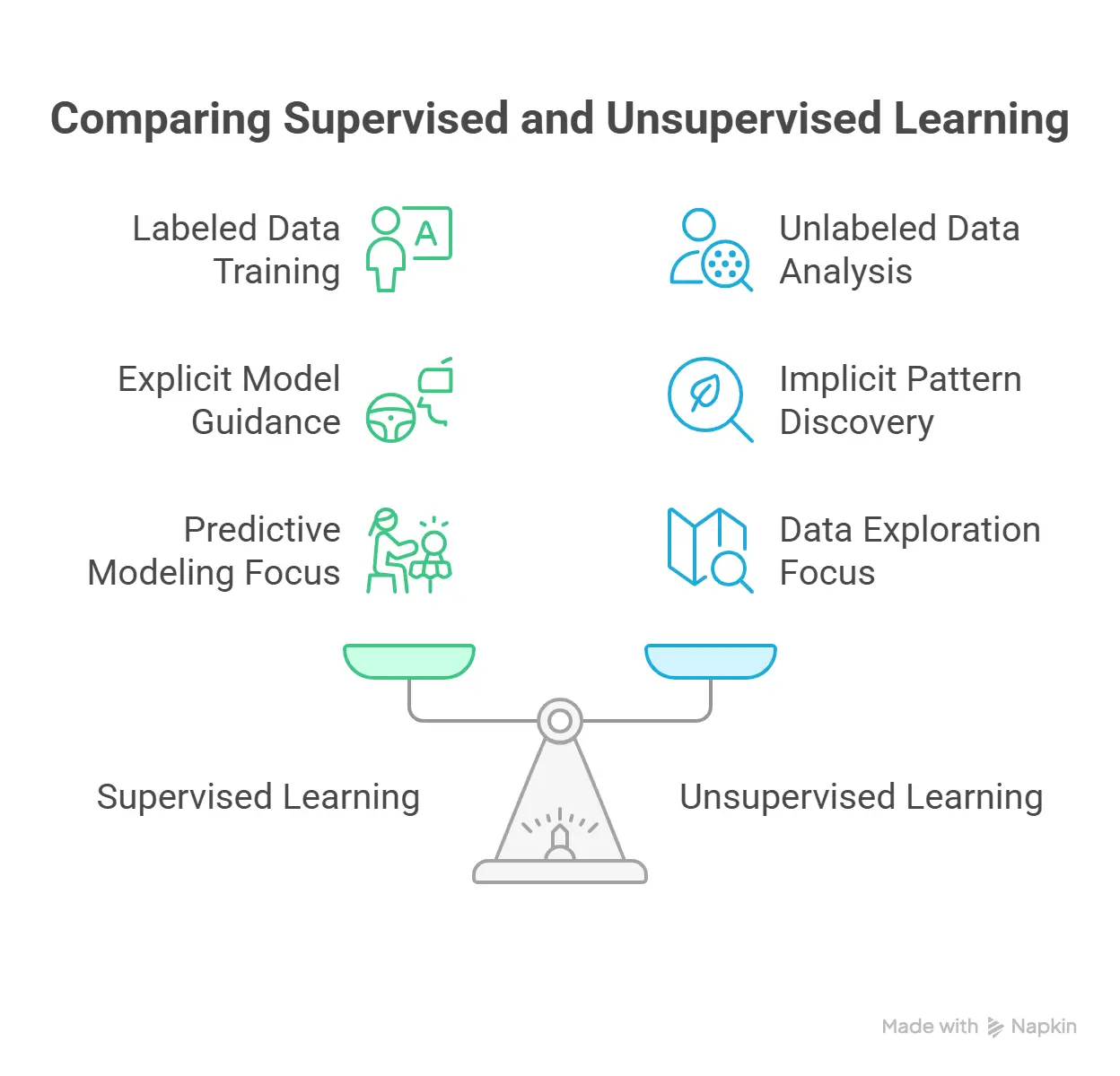
The most salient difference between supervised and unsupervised learning is the type of data utilized for training.

Supervised learning fundamentally relies on labeled data, where each input is explicitly paired with a known correct output.

Conversely, unsupervised learning operates on unlabeled data, discovering inherent patterns and structures without any predefined target outputs.

This core distinction cascades into differing goals, applications, and operational characteristics.

The differing requirements for human intervention represent a critical trade-off. Supervised learning demands substantial upfront human effort for labeling data, which can be costly and time-consuming.

However, this investment yields highly accurate and interpretable predictions, as the model's learning is explicitly guided by correct answers. Conversely, unsupervised learning requires significantly less upfront labeling, making it more flexible for raw data.

Yet, its results are often less predictable and interpretable, as there is no "ground truth" to validate against, leading to outcomes that can be "mostly subjective". This inverse relationship between upfront human effort and post-learning interpretability is a critical decision point in real-world machine learning projects.

Organizations must carefully weigh the cost of data labeling against their need for transparent, verifiable, and precise outcomes. This fundamental trade-off further justifies the emergence of hybrid approaches, which seek to optimize this balance by leveraging both labeled and unlabeled data.

Strengths and weaknesses comparison

The comparative analysis of supervised and unsupervised learning reveals distinct strengths and weaknesses that guide their appropriate application:

Supervised Learning Strengths:

• High Accuracy: Achieves very high predictive accuracy on new, unseen data due to learning from labeled examples.

• Clear Objectives: Provides a clear target for the model, enabling straightforward performance measurement using defined metrics.

• Feature Learning Efficiency: Can identify and prioritize the most crucial features for accurate predictions, optimizing the learning process.

• Robust in Defined Problems: Excels in environments where problems are well-defined and input-output relationships are stable.

• Mature Algorithms: Benefits from a wide array of well-understood and established algorithms.

Supervised Learning Weaknesses:

• Data Dependency: Heavily relies on large, high-quality, and expensive-to-acquire labeled datasets.

• Generalization Issues: Can struggle with generalization to complex or significantly different unseen data, leading to overfitting.

• Bias Vulnerability: Susceptible to inaccuracies and biases present in the labeled training data.

• Computational Cost: Training models, especially deep learning ones, can be computationally intensive.

Unsupervised Learning Strengths:

• No Labeled Data Needed: Can work with vast amounts of raw, unlabeled data, bypassing costly manual labeling.

• Hidden Pattern Discovery: Capable of identifying previously unknown patterns, structures, and novel insights in data.

• Flexibility: Adaptable to various domains where labels are difficult or impractical to obtain.

• Scalability: Highly scalable for processing large datasets without the labeling bottleneck.

• Exploratory Analysis: Excellent for initial data exploration and understanding underlying data structure.

Unsupervised Learning Weaknesses:

• Difficult Evaluation: Lack of ground truth makes objective evaluation of results challenging; outcomes can be subjective.

• Less Interpretability: Results can be less predictable and harder to interpret due to the absence of explicit guidance.

• Noise Sensitivity: Prone to overfitting by capturing noise or spurious patterns in the data.

• Tuning Requirements: Often requires careful and time-consuming parameter tuning to achieve meaningful results.

• Limited for Specific Predictions: May be less effective for complex pattern recognition tasks where clear labels could exist, lacking the explicit guidance of supervised methods.

When to Choose Which Approach

The decision between employing supervised or unsupervised learning hinges on several critical factors, primarily the nature of the problem, the availability and characteristics of the data, and the desired outcome.

1. Data Availability

• The most straightforward determinant is whether labeled data is available. If a high-quality, sufficiently large labeled dataset exists, supervised learning is generally the preferred choice due to its high accuracy and clear performance metrics.
• If data is largely unlabeled, or if labeling is prohibitively expensive or time-consuming, unsupervised learning becomes a more viable, and often necessary, alternative.

2. Problem Type and Goals:

• Supervised learning is ideal when the objective is to predict a specific, known outcome or classify data into predefined categories.
• Examples include predicting a continuous value (e.g., house prices) or a discrete category (e.g., spam email).
• It is chosen when the desired output is clear and measurable.
• Unsupervised learning is suited for exploratory analysis, when the goal is to discover hidden patterns, structures, or relationships within the data without predefined outcomes.
• This includes tasks like grouping customers based on behavior (clustering) or identifying anomalies (anomaly detection). It is used to unearth insights rather than make specific predictions.

3. Required Accuracy and Interpretability

• For applications demanding high accuracy and verifiable results, such as medical diagnosis or fraud detection, supervised learning is typically favored, as its performance can be rigorously evaluated against ground truth.
• When the underlying structure of complex datasets is not well understood, and the aim is to extract hidden patterns that are difficult to recognize, unsupervised learning is more appropriate, even if its results might be less immediately interpretable or quantifiable.

4. Computational Resources and Expertise

• Supervised learning, especially with large datasets, can be computationally intensive during training.
• Unsupervised learning, while avoiding labeling costs, can also demand significant computational power for complex models or very large unclassified datasets.
• The choice also depends on the team's expertise in algorithm selection, parameter tuning, and result interpretation, particularly for unsupervised methods where validation can be more challenging.

Ultimately, the choice between supervised and unsupervised learning is not always mutually exclusive.

In many advanced applications, a hybrid approach, leveraging the strengths of both, often yields the most effective and scalable solutions.

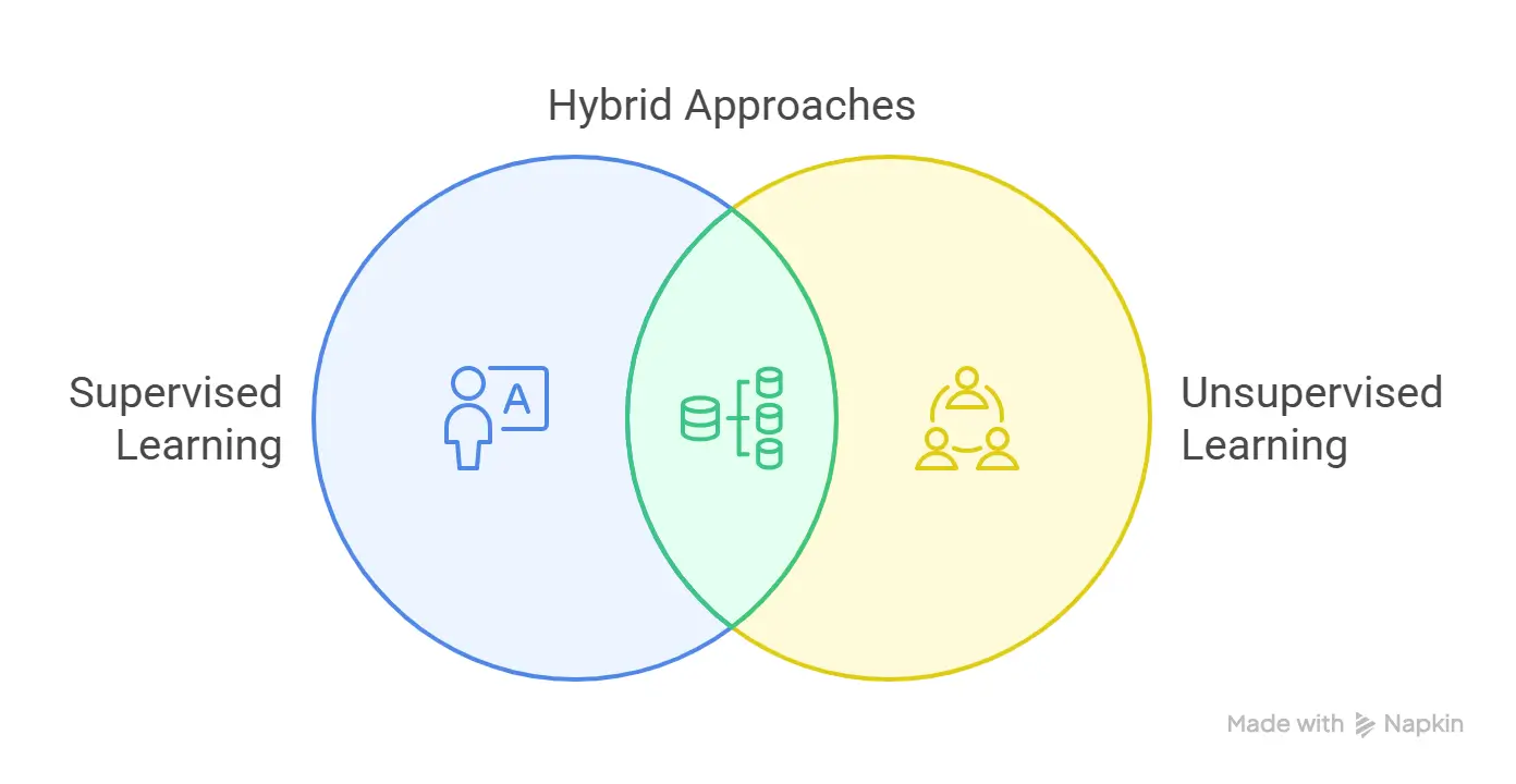
Hybrid approaches

The limitations of purely supervised (high labeling cost) and purely unsupervised (difficult validation and interpretability) learning have spurred the development of hybrid approaches.

These methodologies strategically combine elements from both paradigms to overcome individual shortcomings, particularly in scenarios where labeled data is scarce but unlabeled data is abundant.

These hybrid models represent a crucial evolution in machine learning, offering enhanced accuracy, robustness, interpretability, scalability, and flexibility.

Semi-supervised learning

Semi-supervised learning (SSL) acts as a bridge between supervised and unsupervised learning, utilizing both a small amount of labeled data and a large amount of unlabeled data for model training.

This approach is particularly valuable when manual labeling is expensive or time-consuming, yet vast quantities of unlabeled data are readily available.

The core mechanism of SSL often involves an iterative two-step process. First, an initial model is trained on the small labeled dataset, similar to supervised learning.

This partially trained model then makes predictions (often called "pseudo-labels") on the larger unlabeled dataset.

These pseudo-labeled data points, especially those with high prediction confidence, are then incorporated back into the training process, allowing the model to continuously refine its understanding and improve its accuracy.

This iterative refinement maximizes learning efficiency while minimizing the need for extensive manual labeling.

SSL methods often rely on certain assumptions about the data distribution to effectively leverage unlabeled data:

• Continuity Assumption: Data points that are close to each other in the feature space are likely to share the same output label.

• Cluster Assumption: Data can be naturally divided into discrete clusters, and points within the same cluster are likely to belong to the same class.

• Low-Density Separation Assumption: Decision boundaries between different classes tend to lie in regions of low data density.

Common techniques employed in SSL include:

• Self-training: The model iteratively labels its own unlabeled data based on its current predictions.

• Co-training: Two or more classifiers are trained on different, complementary views of the data. Each classifier then uses its confident predictions on unlabeled data to augment the training set for the other classifiers.

• Graph-based methods: Data points are represented as nodes in a graph, with edges representing relationships. Labels are then propagated through this graph from labeled to unlabeled nodes based on connectivity.

The advantages of SSL are significant: it substantially reduces data labeling costs, enhances model performance (often achieving higher accuracy than purely supervised methods with limited labeled data), and improves generalization by allowing the model to better understand the underlying data structure from unlabeled examples.

It is also highly effective for unstructured data modalities like text, audio, and video. However, SSL also faces challenges, such as the potential for error propagation from initial pseudo-labels, the need for careful selection of high-quality unlabeled data, increased computational complexity for some methods, and a lack of strong theoretical guarantees compared to fully supervised learning.

Applications of semi-supervised learning are diverse:

• Text and Image Classification: Training models with limited labeled data for tasks like celebrity recognition or categorizing text documents.

• Speech Analysis: Overcoming the intensive task of labeling audio files, improving speech recognition models.

• Internet Content Classification: Classifying vast amounts of web content, with search algorithms leveraging SSL to rank webpage relevance.

• Medical Image Analysis: Detecting abnormalities in MRI and CT scans, where labeled medical data is scarce and expensive.

• Customer Segmentation and Anomaly Detection: Applying SSL to improve these tasks by leveraging unlabeled customer data or sensor data.

Self-supervised learning

Self-supervised learning (SSL) is a cutting-edge machine learning technique that leverages the inherent structure within vast amounts of unlabeled data to generate its own supervisory signals, effectively creating implicit labels.

This innovative approach transforms what would conventionally be an unsupervised problem into a supervised one, without requiring any manual human annotation. SSL is particularly impactful in fields like computer vision and natural language processing (NLP), where state-of-the-art AI models traditionally demand prohibitively large and costly labeled datasets.

The core of SSL lies in defining a "pretext task". A pretext task is an artificial, auxiliary task designed such that solving it compels the model to learn useful, high-level representations (features) of the unstructured input data.

These representations, once learned, can then be transferred and fine-tuned for various "downstream tasks," which are the actual real-world problems of interest.

The model is optimized using a loss function, similar to supervised learning, but the "ground truth" for this loss is implicitly derived from the unlabeled input data itself.

Examples of pretext tasks across different modalities include:

1. Image-Based Pretext Tasks:

• Image Inpainting: Masking parts of an image and training the model to predict or reconstruct the missing pixels. This forces the model to understand object structures and textures.
• Contrastive Learning (e.g., SimCLR): Learning representations by minimizing the distance between augmented versions of the same image (positive pairs) and maximizing distance to different images (negative pairs) in the embedding space.
• Predicting Image Rotation: Rotating an image by a random angle and training the model to predict that angle. This helps the model learn object orientation.
• Jigsaw Puzzle: Shuffling image patches and training the model to predict their correct arrangement, thereby learning spatial relationships.

2. Text-Based Pretext Tasks:

• Masked Language Modeling (MLM): Masking random words in a sentence and training the model to predict the missing words based on context.
• This is famously used in models like BERT.
• Next Sentence Prediction (NSP): Training the model to predict whether one sentence logically follows another, learning contextual relationships and coherence.

3. Audio-Based Pretext Tasks:

• Audio Frame Prediction: Masking random frames in an audio waveform and predicting the missing frames, learning temporal dependencies.
• Contrastive Predictive Coding (CPC): Predicting future frames in an audio sequence by contrasting true future frames with negative samples, learning high-level representations of temporal sequences.

The primary advantage of SSL is its ability to learn powerful, general-purpose feature representations from nearly unlimited unlabeled data, significantly reducing the dependence on expensive manual labeling.

This makes it highly cost-effective and scalable, especially for large deep learning models like Large Language Models (LLMs) such as GPT and BERT, which are pre-trained extensively using SSL before fine-tuning for specific tasks.

Transfer learning

Transfer learning (TL) is a machine learning technique where knowledge gained from training a model on one task or dataset (the "source task") is effectively transferred and applied to improve performance on a different, but related, task or dataset (the "target task").

The core idea is to leverage the fundamental knowledge and patterns identified by a pre-trained model, rather than training a new model from scratch, which is typically a time-consuming, computationally intensive process requiring vast amounts of data.

How Transfer Learning Works:

A pre-trained model, often a deep neural network, has already learned a rich set of features and representations from a large, general dataset (e.g., ImageNet for image classification, or a massive text corpus for language models).

In transfer learning, this pre-trained model retains its fundamental knowledge, including its learned features, weights, and functions. This allows it to adapt to new, related tasks much faster and with significantly less data than would be required for de novo training.

The process generally involves three main steps:

1. Select a Pre-trained Model: Choose a model that has already been trained on a large dataset for a task related to the new target task.

2. Feature Extraction or Fine-Tuning:

• Feature Extraction: The pre-trained model's early layers (which learn general features) are used as a fixed feature extractor.

  Only the final layers of the model are retrained on the new, smaller dataset. This is computationally less expensive and suitable when the new dataset is small or the tasks are very similar.

• Fine-Tuning: A more extensive approach where some or all of the pre-trained model's layers are unfrozen and retrained (adjusted) on the new dataset.

  This allows for greater adaptation to the specifics of the new task but requires more data and computational resources. While "transfer learning" is often used broadly, "fine-tuning" specifically refers to this process of retraining parts of a pre-trained model.

Types of Transfer Learning:

• Inductive Transfer Learning: Source and target tasks are different, but the source data might be labeled. Models pre-trained for feature extraction on large datasets are adapted for specific tasks like object detection. Multitask learning (simultaneously learning two tasks on the same dataset) is a form of inductive transfer.

• Transductive Transfer Learning: Knowledge is transferred from a specific source domain to a different but related target domain, with a focus on the target domain. Useful when there's little or no labeled data in the target domain, but the target data is mathematically similar to the source.

• Unsupervised Transfer Learning: Both source and target domains have unlabeled data. The model learns common features to generalize more accurately for a target task.

Advantages of Transfer Learning:

• Reduced Computational Costs: Significantly lowers the computational resources (training time, data, processing power) required to build models for new problems.

• Alleviates Data Scarcity: Particularly beneficial when acquiring large, manually labeled datasets for the target task is difficult or expensive.

• Improved Performance and Generalizability: Models often demonstrate greater robustness and better performance in diverse, real-world environments, having learned from a wider variety of scenarios during initial training. This can also inhibit overfitting.

Transfer learning is a critical strategy in generative AI, allowing organizations to customize large foundation models without training new ones from scratch, saving immense computational resources and time.

For example, a large language model (LLM) pre-trained on a massive text corpus can be fine-tuned for specific NLP tasks like sentiment analysis with a much smaller, task-specific dataset.

Advantages of Hybrid Machine Learning Architectures

Hybrid machine learning architectures, by blending traditional ML techniques with deep learning strategies or combining multiple models in layered or parallel configurations, offer compelling advantages over single-model solutions.

These benefits stem from their ability to leverage the complementary strengths of different learning paradigms:

• Higher Predictive Accuracy: By integrating diverse component models, each focusing on specific aspects or types of data (e.g., traditional ML for structured data, deep learning for unstructured text/images), hybrid systems can combine their strengths to deliver more reliable and accurate predictions across varied datasets.

  This synergistic effect often leads to superior performance compared to any single model approach.

• Greater Robustness: Hybrid systems are designed to handle a wider variety of data types and tasks, making them highly adaptable to real-world variability and noise.

  They can integrate multiple approaches to ensure consistent results even in changing conditions or when dealing with incomplete data, leading to more resilient models.

Conclusion and Future Outlook

The landscape of machine learning is fundamentally shaped by two primary paradigms: supervised learning and unsupervised learning. Supervised learning, with its reliance on meticulously labeled data, excels in predictive tasks where clear, verifiable outcomes are required.

Its "teacher-guided" approach ensures high accuracy and reliability in well-defined problems, making it indispensable for critical applications such as fraud detection, medical diagnosis, and precise forecasting.

However, this precision comes at the significant cost of extensive and often expensive data labeling, a bottleneck that limits its scalability and applicability in data-rich but label-poor environments.

Conversely, unsupervised learning thrives in the absence of labels, autonomously discovering hidden patterns, structures, and insights within raw data. Its "self-discovery" nature makes it invaluable for exploratory data analysis, customer segmentation, anomaly detection, and dimensionality reduction.

While offering unparalleled flexibility and scalability for vast datasets, unsupervised learning faces challenges in objective evaluation and interpretability due to the lack of ground truth. The insights it unearths are often hypothesis-generating rather than definitive predictions, requiring careful human interpretation.

The inherent limitations of purely supervised and unsupervised approaches have propelled the field towards innovative hybrid methodologies.

Semi-supervised learning effectively bridges this gap by leveraging a small amount of labeled data to guide the learning process on a much larger pool of unlabeled data, significantly reducing labeling costs while enhancing model performance and generalization.

Self-supervised learning takes this a step further, generating its own supervisory signals from the data itself through "pretext tasks," enabling models to learn powerful representations from massive unlabeled datasets, a breakthrough for areas like computer vision and natural language processing. Complementing these, transfer learning allows knowledge acquired from one task to be repurposed for related tasks, drastically cutting down training time and data requirements for new applications.

These hybrid architectures represent a mature evolution of machine learning, demonstrating higher predictive accuracy, greater robustness, improved interpretability, and enhanced scalability. They collectively address the "cost of knowledge" inherent in data annotation, pushing the boundaries of what is possible by making more efficient use of the abundant unlabeled data in the world.

The future outlook for machine learning points towards a continued emphasis on these hybrid and adaptive learning paradigms. As data volumes continue to explode, and the demand for intelligent systems grows across increasingly complex and dynamic domains, the ability to learn effectively from diverse data sources—both labeled and unlabeled—will be paramount.

Research will likely focus on developing more sophisticated self-supervised pretext tasks, refining semi-supervised algorithms for even greater data efficiency, and exploring novel ways to combine and transfer knowledge across different modalities and tasks.

The pursuit of more generalized, robust, and autonomous learning systems, capable of extracting meaningful information from the raw complexity of the real world, will define the next frontier of machine intelligence.