Best Machine Learning Libraries
In the ever-evolving landscape of machine learning and artificial intelligence, a solid grasp of both theory and practical tools is essential. This guide delves into the top machine learning libraries, exploring their theoretical foundations alongside practical applications. Whether you're a seasoned data scientist or an aspiring ML engineer, this comprehensive overview will deepen your understanding and enhance your toolkit.
Machine learning has revolutionized the field of data analysis and predictive modelling. With the help of machine learning libraries, developers and data scientists can easily implement complex algorithms and models without writing extensive code from scratch. In this article, we will explore the top 7 libraries for machine learning and understand their features, use cases, pros, and cons. Whether you are a beginner or an experienced professional, these deep learning libraries will undoubtedly enhance your machine-learning capabilities.
The rapidly evolving field of machine learning has given rise to a plethora of powerful libraries, each offering unique strengths and capabilities. From the versatility of TensorFlow and PyTorch to the specialized efficiency of XGBoost and LightGBM, these libraries have become indispensable tools for data scientists and researchers alike. Whether you're building complex neural networks, tackling large-scale regression problems, or exploring cutting-edge techniques in computer vision, there's a library out there that can help you achieve your goals.
scikit-learn

Scikit-learn is built on the principle of consistent interfaces across various machine learning algorithms. It implements a wide range of supervised and unsupervised learning algorithms based on a set of well-established mathematical and statistical models.
Real-world application
Scikit-learn is widely used in various industries for tasks like customer churn prediction, spam detection, and medical diagnosis. Its versatility makes it a go-to choice for many data scientists tackling diverse problems.
Key Concepts
Estimators: The core concept in scikit-learn. Any object that can estimate some parameters based on a dataset is considered an estimator.
Transformers: Estimators that can transform input data are called transformers.
Predictors: Estimators capable of making predictions are called predictors.
Meta-estimators: These estimators can be based on other estimators, like ensemble methods.
Key features
Easy-to-use interface
Comprehensive documentation and examples
Built on NumPy, SciPy, and matplotlib
Great for preprocessing, model selection, and evaluation
Example
This code loads the Iris dataset and splits it into training and testing sets. A Random Forest classifier is trained on the training data, and predictions are made on the test data. Finally, it calculates and prints the model's accuracy, indicating how well it classifies the iris species.
from sklearn.datasets import load_iris
from sklearn.model_selection import train_test_split
from sklearn.ensemble import RandomForestClassifier
from sklearn.metrics import accuracy_score

# Load the iris dataset
iris = load_iris()
X, y = iris.data, iris.target

# Split the data
X_train, X_test, y_train, y_test = train_test_split(X, y, test_size=0.3, random_state=42)

# Train a Random Forest classifier
clf = RandomForestClassifier(n_estimators=100)
clf.fit(X_train, y_train)

# Make predictions and evaluate
predictions = clf.predict(X_test)
print(f"Accuracy: {accuracy_score(y_test, predictions):.2f}")
TensorFlow

TensorFlow is based on the concept of computational graphs, where nodes represent mathematical operations and edges represent multidimensional data arrays (tensors) communicated between them. This approach allows for efficient computation and automatic differentiation, which is crucial for training deep neural networks.
Real-world application
TensorFlow powers numerous applications, from Google Translate to autonomous vehicles and medical imaging analysis. Its scalability makes it suitable for both research and production environments.
Key Concepts
Tensors: Multidimensional arrays that form the basic data structure in TensorFlow.
Computational Graphs: A series of TensorFlow operations arranged into a graph of nodes.
Automatic Differentiation: The ability to automatically compute gradients, which is essential for backpropagation in neural networks.
Eager Execution: A define-by-run interface where operations are executed immediately.
Key features
Flexible ecosystem for building and deploying ML models
Supports both CPU and GPU computing
TensorFlow Lite for mobile and embedded devices
Keras integration for high-level neural network APIs
Example
This code builds and trains a simple feedforward neural network using TensorFlow and Keras. The model consists of two hidden layers with ReLU activation and an output layer with a sigmoid activation for binary classification. It is compiled with the Adam optimizer and binary cross-entropy loss, and then trained on the training data (X_train, y_train) for 10 epochs, using 20% of the data for validation.
import tensorflow as tf
from tensorflow.keras.models import Sequential
from tensorflow.keras.layers import Dense

# Create a simple feedforward neural network
model = Sequential([
    Dense(64, activation='relu', input_shape=(10,)),
    Dense(32, activation='relu'),
    Dense(1, activation='sigmoid')
])

model.compile(optimizer='adam', loss='binary_crossentropy', metrics=['accuracy'])

# Assuming X_train and y_train are your training data
model.fit(X_train, y_train, epochs=10, batch_size=32, validation_split=0.2)
PyTorch
PyTorch is built on the concept of dynamic computation graphs, which allows for more flexible and intuitive model building. This approach is particularly beneficial for tasks that require variable-length inputs or complex control flow.
Real-world application
PyTorch is extensively used in computer vision tasks, natural language processing, and reinforcement learning research. Its flexibility makes it particularly popular in academic and research settings.
Key Concepts
Dynamic Computational Graphs: Graphs are built on-the-fly, allowing for more dynamic and flexible model structures.
Autograd: Automatic differentiation engine that supports all differentiable tensor operations.
Torch.nn: A module to help create and train neural networks.
JIT (Just-In-Time) Compilation: Allows for optimizing and serializing models.
Key features
Dynamic computational graphs
Intuitive debugging
Strong community support
Excellent for natural language processing tasks
Example
This code defines a simple neural network using PyTorch, consisting of two fully connected layers with ReLU and sigmoid activations for binary classification. It initializes the model, binary cross-entropy loss function, and Adam optimizer. A training loop runs for 100 epochs, where it computes the model's outputs, calculates the loss, performs backpropagation, and updates the model parameters based on the gradients.
import torch
import torch.nn as nn
import torch.optim as optim

# Define a simple neural network
class SimpleNet(nn.Module):
    def __init__(self):
        super(SimpleNet, self).__init__()
        self.fc1 = nn.Linear(10, 5)
        self.fc2 = nn.Linear(5, 1)

    def forward(self, x):
        x = torch.relu(self.fc1(x))
        x = torch.sigmoid(self.fc2(x))
        return x

# Initialize the model, loss function, and optimizer
model = SimpleNet()
criterion = nn.BCELoss()
optimizer = optim.Adam(model.parameters())

# Training loop (assuming X_train and y_train are your training data)
for epoch in range(100):
    optimizer.zero_grad()
    outputs = model(X_train)
    loss = criterion(outputs, y_train)
    loss.backward()
    optimizer.step()
XGBoost

XGBoost is based on the gradient boosting framework, a powerful ensemble technique. It builds sequential trees, where each tree corrects the errors of the previous ones.
Real-world application
XGBoost is widely used in finance for credit scoring, in retail for sales forecasting, and in healthcare for predicting patient outcomes. Its ability to handle complex relationships in data makes it a top choice for many Kaggle competitions.
Key Concepts
Gradient Boosting: An ensemble technique that combines weak learners (typically decision trees) to create a strong predictor.
Regularization: XGBoost includes L1 and L2 regularization to prevent overfitting.
Parallel Processing: Utilizes parallel processing for tree building and evaluation.
Sparsity-aware Split Finding: Efficiently handles missing values and sparse data.
Key features
High performance and fast execution
Regularization to prevent overfitting
Handles missing values automatically
Parallel and distributed computing support
Example
This code generates a synthetic regression dataset and splits it into training and testing sets. It creates DMatrix objects for efficient data handling with XGBoost, sets model parameters for training (including maximum depth and learning rate), and trains the model for 100 rounds. Finally, it uses the trained model to make predictions on the test data.
import xgboost as xgb
from sklearn.datasets import make_regression
from sklearn.model_selection import train_test_split

# Create a synthetic regression dataset
X, y = make_regression(n_samples=1000, n_features=20, noise=0.1)
X_train, X_test, y_train, y_test = train_test_split(X, y, test_size=0.2)

# Create DMatrix for XGBoost
dtrain = xgb.DMatrix(X_train, label=y_train)
dtest = xgb.DMatrix(X_test, label=y_test)

# Set parameters
params = {
    'max_depth': 3,
    'eta': 0.1,
    'objective': 'reg:squarederror',
    'eval_metric': 'rmse'
}

# Train the model
num_rounds = 100
model = xgb.train(params, dtrain, num_rounds)

# Make predictions
predictions = model.predict(dtest)
Keras
Keras is designed with user-friendliness as its core principle. It provides a high-level API for building neural networks, abstracting away many of the complexities involved in deep learning.
Real-world application
Keras is popular for image classification tasks, sentiment analysis, and building chatbots. Its simplicity makes it a favorite for rapid prototyping and for those new to deep learning.
Key Concepts
Sequential and Functional APIs: Two ways to define models, offering flexibility in network architecture design.
Layers: Building blocks of neural networks, each with its own set of weights and computations.
Models: A way to organize layers and define inputs and outputs.
Callbacks: Functions to apply during training for customizing the training process.
Key features
High-level neural networks API
Runs on top of TensorFlow, Theano, or CNTK
Fast prototyping
Supports both convolutional and recurrent networks
Example
This code defines a convolutional neural network (CNN) using TensorFlow and Keras for image classification. It consists of two convolutional layers (with ReLU activation) followed by max pooling layers, which reduce spatial dimensions. After flattening the output, it includes two dense layers, with the final layer using softmax activation to output probabilities for 10 classes. The input shape is set for grayscale images of size 28x28 pixels.
from tensorflow.keras.models import Sequential
from tensorflow.keras.layers import Conv2D, MaxPooling2D, Flatten, Dense

model = Sequential([
    Conv2D(32, (3, 3), activation='relu', input_shape=(28, 28, 1)),
    MaxPooling2D((2, 2)),
    Conv2D(64, (3, 3), activation='relu'),
    MaxPooling2D((2, 2)),
    Flatten(),
    Dense(64, activation='relu'),
    Dense(10, activation='softmax')
])
NLTK (Natural Language Toolkit)
NLTK is built on linguistic principles and provides tools for various NLP tasks. It incorporates theories from computational linguistics to process and analyze human language data.
Real-world application
NLTK is used in sentiment analysis for social media monitoring, chatbot development, and automated content categorization. Its comprehensive toolkit makes it valuable for both academic research and practical NLP applications.
Key Concepts
Tokenization: Breaking text into individual words or sentences.
Part-of-Speech Tagging: Assigning grammatical tags to words.
Named Entity Recognition: Identifying and classifying named entities in text.
Stemming and Lemmatization: Reducing words to their root form.
Key features
Extensive suite of text processing libraries
Includes corpora and lexical resources
Supports classification, tokenization, stemming, tagging, and parsing
Example
This code uses NLTK to perform basic natural language processing tasks on a given text. It first tokenizes the text into words, then removes common English stopwords, which are insignificant for analysis. Finally, it applies stemming using the Porter stemmer to reduce words to their root forms. The resulting stemmed tokens are printed out.
import nltk
from nltk.tokenize import word_tokenize
from nltk.corpus import stopwords
from nltk.stem import PorterStemmer

# Download necessary NLTK data
nltk.download('punkt')
nltk.download('stopwords')

text = "Natural language processing is fascinating. It helps computers understand human language."

# Tokenize
tokens = word_tokenize(text)

# Remove stopwords
stop_words = set(stopwords.words('english'))
filtered_tokens = [word for word in tokens if word.lower() not in stop_words]

# Stemming
stemmer = PorterStemmer()
stemmed_tokens = [stemmer.stem(word) for word in filtered_tokens]
print(stemmed_tokens)
Pandas

Pandas is built on the concept of data frames, similar to those in R. It provides data structures and operations for manipulating numerical tables and time series.
Real-world application
Pandas is used extensively in financial analysis, scientific computing, and as a preprocessing step in most machine learning pipelines. Its ability to handle various data formats makes it invaluable for data cleaning and preparation tasks.
Key Concepts
DataFrame: 2-dimensional labeled data structure with columns of potentially different types.
Series: 1-dimensional labeled array capable of holding data of any type.
Index: Immutable array-like object for labeling axes.
GroupBy: Split-apply-combine operations for aggregating data.
Key features
Efficient data structures (DataFrame, Series)
Powerful data manipulation and merging capabilities
Integrated time series functionality
Handles missing data
Example
This code creates a sample Pandas DataFrame with three columns: 'A' (random floats), 'B' (random integers), and 'C' (categorical strings). It then performs basic operations: `describe()` provides summary statistics of the numeric columns, `groupby()` calculates the mean of column 'A' for each category in 'C', and `sort_values()` sorts the DataFrame by column 'B' in descending order.
import pandas as pd
import numpy as np

# Create a sample DataFrame
df = pd.DataFrame({
    'A': np.random.rand(5),
    'B': np.random.randint(0, 10, 5),
    'C': ['foo', 'bar', 'baz', 'qux', 'quux']
})

# Basic operations
print(df.describe())
print(df.groupby('C').mean())
print(df.sort_values(by='B', ascending=False))
Matplotlib and Seaborn: Data Visualization
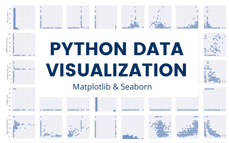
Matplotlib is based on MATLAB's plotting interface and focuses on creating static, animated, and interactive visualizations in Python. Seaborn, built on top of Matplotlib, incorporates statistical graphics and aesthetics based on principles of effective data visualization.
Real-world application
These libraries are used for creating insightful visualizations in data science reports, academic papers, and business presentations. They play a crucial role in exploratory data analysis and communicating results effectively.
Key Concepts
Figure and Axes: The main concepts in Matplotlib for organizing plots.
Statistical Graphics: Seaborn provides high-level interfaces for statistical graphics.
Color Palettes: Carefully chosen color schemes in Seaborn for effective data representation.
Grammar of Graphics: Seaborn follows some principles from the "Grammar of Graphics" concept.
Key features
Wide range of plot types
Customizable aesthetics
Integration with Pandas
Statistical data visualization (Seaborn)
Example
This code uses Matplotlib and Seaborn to create two visualizations. The first plot displays a sine wave using Matplotlib, with labeled axes and a title. The second plot uses Seaborn to create a scatter plot of the "tips" dataset, showing the relationship between total bill and tip amount, color-coded by dining time (lunch or dinner). Both visualizations are presented with appropriate styles and titles.
import matplotlib.pyplot as plt
import seaborn as sns
import numpy as np

# Sample data
x = np.linspace(0, 10, 100)
y = np.sin(x)

# Matplotlib plot
plt.figure(figsize=(10, 4))
plt.plot(x, y)
plt.title('Sine Wave')
plt.xlabel('x')
plt.ylabel('sin(x)')
plt.show()

# Seaborn plot
sns.set_style("whitegrid")
tips = sns.load_dataset("tips")
sns.scatterplot(x="total_bill", y="tip", hue="time", data=tips)
plt.title('Tips vs Total Bill')
plt.show()
Conclusion
The machine learning ecosystem is rich with powerful libraries, each offering unique strengths and theoretical foundations. This guide has explored the underlying concepts and practical applications of eight key libraries:
Scikit-learn: Versatile machine learning algorithms
TensorFlow: Deep learning with computational graphs
PyTorch: Dynamic computation graphs for flexible deep learning
XGBoost: Advanced gradient boosting
Keras: User-friendly neural network API
NLTK: Comprehensive natural language processing
Pandas: Efficient data manipulation and analysis
Matplotlib and Seaborn: Statistical data visualization
Understanding both the theoretical underpinnings and practical usage of these libraries is crucial for any data scientist or ML engineer. The choice of library depends on various factors including the specific problem, data scale, computational resources, and deployment environment.
As the field continues to evolve, new libraries and tools will emerge, and existing ones will improve. Continuous learning and hands-on practice are key to staying at the forefront of this exciting field.
Remember, mastering these libraries goes beyond syntax knowledge. It requires understanding their underlying principles, strengths, and limitations. By combining theoretical knowledge with practical skills, you'll be well-equipped to tackle a wide range of machine learning challenges.
