


Implementing a Convolutional Neural Network with Python


A Convolutional Neural Network (CNN) is a type of deep learning model specifically designed to automatically detect patterns in visual data, such as images. It achieves this by applying filters that extract features like edges, textures, and shapes, which are then used to make predictions based on these features.
CNNs are significant in the field of artificial intelligence because they can learn visual patterns directly from data, eliminating the need for manual feature extraction. This capability makes them highly effective for tasks that require an understanding of images or spatial data.
They are widely used in various applications, including image recognition (identifying objects in photos), medical imaging (detecting diseases from scans), face recognition systems, and self-driving cars (which detect lanes, pedestrians, and traffic signs).
For instance, when you upload a photo to social media, and it automatically tags people or suggests objects in the image, this functionality is powered by CNNs, which analyze visual features step by step.
Why CNN is the Best Choice for Image Data
Traditional neural networks (ANNs) struggle with image data because they treat every pixel as an independent input. This approach ignores the spatial relationships between neighboring pixels and leads to a massive number of parameters, making models inefficient and more prone to overfitting.
Images, however, are inherently spatial data; nearby pixels are connected and together form meaningful patterns such as edges, textures, and shapes. To truly understand images, a model must preserve these relationships instead of flattening them into a single vector.
Convolutional Neural Networks (CNNs) are specifically designed to handle this challenge. By maintaining spatial structure and learning visual patterns efficiently, they overcome the limitations of traditional neural networks.
Building on this, CNNs introduce key mechanisms that make them highly effective for image data, as outlined below:
1. Local Connectivity
CNNs process small regions of an image at a time, known as receptive fields. This allows the model to first detect simple patterns like edges and corners, and then combine them into more complex features.
2. Parameter Sharing
Instead of learning separate weights for every pixel, CNNs use the same filter (kernel) across the entire image. This significantly reduces the number of parameters and improves computational efficiency.
3. Translation Invariance
CNNs can recognize patterns regardless of their position in the image. An object can be detected whether it appears at the center or the corner, making the model more robust in real-world scenarios.
CNN vs ANN: Key Difference and When to Use Each
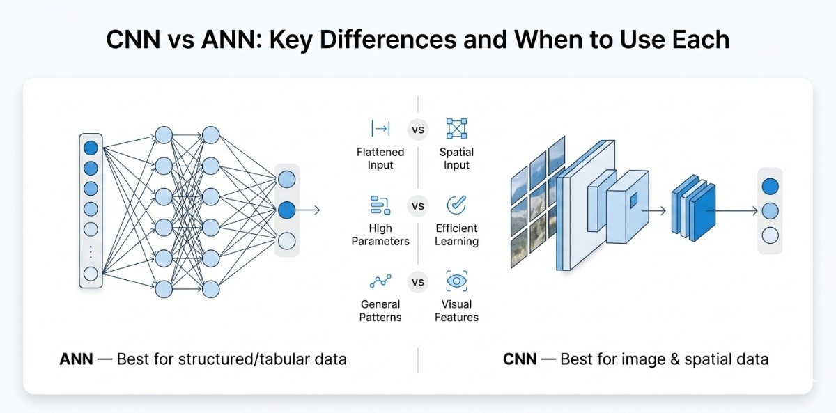
Choosing between Artificial Neural Networks (ANNs) and Convolutional Neural Networks (CNNs) is not just a theoretical decision; it directly influences how effectively your model learns, how efficiently it utilizes resources, and how well it scales with real-world data.
While ANNs are often the starting point for beginners due to their simplicity, they quickly reveal limitations when applied to image or spatial data, where structure and relationships play a critical role.
How ANN Works (Traditional Approach)
An Artificial Neural Network (ANN) treats input data as a flat sequence of numerical values, meaning that even structured data like images is converted into a one-dimensional vector before processing. It is suitable for structured datasets; it fails to retain the inherent relationships between data points when applied to images.
By flattening the input, ANNs lose the spatial context that defines visual information, making it difficult for the model to recognize meaningful patterns such as edges, shapes, or textures.
Additionally, because every input node is connected to every neuron, the number of parameters increases significantly, leading to higher computational cost and a greater risk of overfitting. As a result, ANNs are not well-suited for tasks that require an understanding of visual structure.
How CNN Works (Modern Approach)
A Convolutional Neural Network (CNN) is designed to overcome these limitations by processing data in its original structured form. Instead of flattening the input, CNNs apply filters across the image to capture local patterns and preserve spatial relationships.
This approach allows the model to detect fundamental features such as edges and textures in the early stages, and progressively build more complex representations in deeper layers.
By using shared weights and localized connections, CNNs significantly reduce the number of parameters while improving learning efficiency. This structured way of learning makes CNNs far more effective for tasks that involve images or any form of spatial data.
Key Takeaway and When to Use What
In practical scenarios, ANNs are best suited for problems involving structured or tabular data, where relationships between features are not dependent on position or spatial arrangement. They are simple to implement and perform well when the data does not carry inherent structure.
CNNs, on the other hand, are specifically built for data where spatial relationships matter, such as images and videos. By preserving structure, automatically extracting features, and scaling efficiently with complex inputs, CNNs have become the standard approach for most computer vision tasks.
Choosing between the two ultimately depends on whether your data requires spatial understanding or not.
Prerequisites: What You Need to Know Before Building a CNN
Before you start building a Convolutional Neural Network (CNN), it’s important to have a basic foundation in a few key areas. You don’t need deep expertise, but understanding the fundamentals will help you follow the implementation smoothly and avoid unnecessary confusion as you move forward.
From a Python perspective, you should be comfortable with basic programming concepts such as variables, loops, functions, and working with libraries. Since most deep learning frameworks are built in Python, being able to read and understand code is enough to get started.
On the machine learning side, having a high-level understanding of how models learn from data is helpful. Concepts like training and testing, overfitting, and how predictions are made will give you the context needed to understand what your CNN is doing. You don’t need to go deep into the math, just knowing the intuition is sufficient.
In terms of libraries, you will primarily work with TensorFlow and Keras for building and training models, NumPy for handling numerical data, and Matplotlib for visualizing results. These tools form the core environment for most CNN-based projects.
To quickly set up your environment, install the required libraries using:
pip install tensorflow keras numpy matplotlibAfter installing TensorFlow and PyTorch, it’s important to follow the official setup guides for each framework to ensure everything is configured correctly for your system.
If you plan to work on larger datasets or train more complex models, using a GPU is highly recommended. While it is completely optional for beginners and smaller projects, a GPU significantly speeds up training by parallelizing computations, which can otherwise take a long time on a CPU.
Setting up GPU support typically involves installing CUDA and cuDNN, and both TensorFlow and PyTorch provide guidance for this in their official documentation.
Once your environment is properly set up and all required libraries are installed, you’ll be ready to move forward and start building your first CNN model with confidence.
Step by Step Process of How CNN Processes Images
A Convolutional Neural Network (CNN) processes an image through a structured pipeline where raw pixel values are gradually transformed into meaningful predictions. Instead of analyzing the entire image at once, the network first extracts important visual patterns and then uses those learned features to classify the image.
The image we'll use as a running example throughout: a 6×6 grayscale picture of the letter "X". Simple, concrete, and small enough to trace by hand.
The convolution operation: filters and kernels
A convolution layer doesn't look at the whole image at once. It looks at a small patch, does a quick calculation, then slides to the next patch. That's it. The intelligence is in what calculation it does and how it learns to do it better over time.
That small patch detector is called a filter (also called a kernel). A filter is just a tiny grid of numbers, typically 3×3. It slides across the image from left to right, top to bottom. At every position, it multiplies its numbers with the image patch underneath, sums the results, and writes one output number. That output number goes into a new grid called a feature map.
Here's what that looks like in practice. Take a 3×3 edge-detection filter and apply it to a patch of our image:
Image patch (3×3):
1  1  0
1  0  0
0  0  0
Filter (3×3) a simple vertical edge detector:
1  0  -1
1  0  -1
1  0  -1
Dot product (element-wise multiply, then sum):
(1×1) + (1×0) + (0×-1)
(1×1) + (0×0) + (0×-1)
(0×1) + (0×0) + (0×-1)
= 1 + 0 + 0 + 1 + 0 + 0 + 0 + 0 + 0
= 2
That ( 2 ) is written into one cell of the feature map. The filter slides one step right and repeats. This is the convolution operation, nothing more than multiply-and-add, applied systematically across the image.
The key insight: the network doesn't choose what filter values to use. It starts with random values and learns the right values during training through backpropagation. By the end of training, your first layer's filters have naturally evolved to detect edges. Deeper layers detect corners, curves, textures, and eventually entire objects, all by doing this same operation repeatedly.
.svg)
The filter slides across the full image. At each position, it computes one output value via element-wise multiply and sum. A 6×6 image with a 3×3 filter (stride 1, no padding) produces a 4×4 feature map.
One convolution layer doesn't just apply one filter; it applies many. A typical first layer uses 32 filters simultaneously. Each filter looks for something slightly different. One might detect vertical edges, another horizontal edges, and another diagonal lines.
The result is 32 separate feature maps stacked together, giving the next layer a rich description of what's in the image.
Stride and padding (controlling output size)
Two parameters control exactly how the filter slides across the image: stride and padding. Understanding these saves you from one of the most common beginner errors, a shape mismatch that crashes your model before it even starts training.
Stride is how many pixels the filter moves each step. Stride of 1 means the filter moves one pixel at a time (default). Stride of 2 means it jumps two pixels, scanning the image faster but producing a smaller feature map.
Padding controls what happens at the edges. Without padding (valid), the filter can't start at the corners, so the output shrinks. With the same padding, zeros are added around the border so the output stays the same size as the input.
Use this formula to calculate your output size before building a model:
Output size=SW−F+2P/S +1
Where W = input width, F = filter size, P = padding, and S = stride.

In practice, you'll use padding='same' in most of your convolutional layers to prevent the feature maps from shrinking too early. Keep padding='valid' for situations where you deliberately want the spatial dimensions to reduce as depth increases.
Activation function, ReLU, and why it matters
After the convolution step, every value in the feature map gets passed through an activation function. The one you'll see everywhere in CNNs is ReLU, Rectified Linear Unit.
ReLU is almost embarrassingly simple:
f(x) = max(0, x)If the value is positive, keep it. If it's negative, replace it with zero. That's the entire function.
So why does this matter so much? Because convolution is a linear operation, it's just a matter of multiplying and adding. Stack ten linear operations on top of each other, and you still have just one linear operation. Your deep network would be no more powerful than a single layer of math.
ReLU introduces non-linearity. Once you add it, stacking layers gives you genuinely new expressive power at each depth. Your network can now learn curved boundaries, complex shapes, and non-obvious patterns, not just straight lines through data.
It also helps with a nasty problem in older networks called the vanishing gradient. Previous activation functions, like sigmoid, squash all values into a tiny range near 0 or 1.
During backpropagation, gradients are multiplied by dozens of these squashed values, becoming so small that they essentially disappear; the early layers stop learning entirely. ReLU doesn't squash positive values, so gradients flow back cleanly through the network.
model.add(layers.Conv2D(32, (3, 3), activation='relu'))
# activation='relu' applies ReLU to every value in the feature map
# Negative values → 0. Positive values → unchanged..svg)
All negative values in the feature map become 0. Positive value pass through unchanged. This one operation makes deep networks actually learnable.
Pooling layers, max pooling vs average pooling
After convolution and ReLU, your feature maps are still quite large. If you had a 32×32 input image and ran 32 filters, you now have 32 feature maps, each 30×30 in size.
That's 28,800 values, and this is only after the first layer. Without doing something to reduce this, the model becomes computationally unmanageable and prone to memorizing training data instead of generalizing.
The pooling layer is the solution. It shrinks each feature map by summarizing small regions into a single number. The most common version, max pooling, takes a 2×2 window and keeps only the maximum value inside it, then slides two steps to the next window.
Why keep the maximum rather than the average? Because in a feature map, a high value means "this filter found something interesting here." Taking the maximum preserves that signal. Average pooling dilutes it by averaging with nearby weaker responses.
Max pooling is more aggressive and generally works better for image classification. It keeps asking "Did anything interesting happen here?" rather than "What was the average response?"
.svg)
Here's a quick comparison to keep in your back pocket:
In Keras: model.add(layers.MaxPooling2D((2, 2))) This halves both the width and height of every feature map.
Fully connected layer and the flatten operation
At this point in the network, you have a stack of feature maps. Each one is a 2D grid of numbers representing how strongly each filter responded at each location in the image. The problem is that the next part of the network, the classifier, expects a simple one-dimensional list of numbers, not a 3D stack of grids.
The flattened layer bridges this gap. It takes all the feature map values and unrolls them into a single long vector, left to right, top to bottom, through every map.
If your final set of feature maps has shape (8, 8, 64), that's 8×8 spatial resolution with 64 filters, then flattening produces a vector of length 8 × 8 × 64 = 4,096 values.
That 4,096-dimensional vector then feeds into one or more Dense (fully connected) layers. Each neuron in a Dense layer is connected to every value in that vector. This is where the network stops asking "where is the edge?" and starts asking "given everything I detected, what is this image?"
The final Dense layer has exactly as many neurons as the number of classes, 10 for CIFAR-10. It uses softmax activation to convert raw scores into probabilities that sum to 1.
model.add(layers.Flatten())
# Converts (8, 8, 64) → (4096,) — one long vector

model.add(layers.Dense(64, activation='relu'))
# Fully connected — all 4096 inputs connect to all 64 neurons

model.add(layers.Dense(10, activation='softmax'))
# 10 neurons = 10 classes, softmax outputs probabilities.svg)
Putting it all together, the complete CNN data flow
Every concept above is one link in a chain. Let's see the full picture, how data flows from a raw image pixel all the way to a class prediction, layer by layer.

Notice the pattern: spatial dimensions (height × width) shrink as you go deeper, while depth (number of feature maps) grows. This is intentional. Early layers have large feature maps with simple, local features: edges, colors. Later layers have small, compressed feature maps rich with abstract, global features, shapes, and objects. The network trades spatial detail for semantic understanding as data flows forward.
This is exactly the architecture you'll build in the next section. Now that you understand what each layer is doing and why, the code will make complete sense from the first line.
Complete CNN Workflow from Data to Prediction
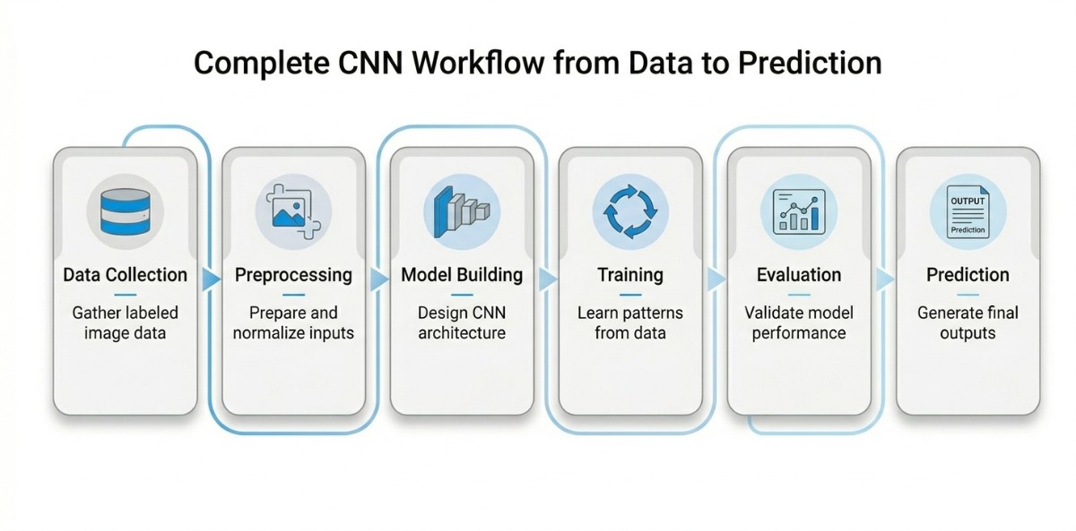
Building a CNN is not just about stacking layers and running code. It is a structured process where each stage plays a critical role in shaping how the model learns and performs. Understanding this workflow helps bridge the gap between theoretical concepts and real-world implementation, making it easier to design models that are both effective and reliable.
Data Collection
The process begins with gathering a dataset that truly represents the problem you want to solve. For image-based tasks, this means collecting labeled images across relevant categories, which involves proper data annotation to ensure accuracy, consistency, and enough variation in lighting, angles, and conditions. The model does not understand context as humans do; it learns entirely from the data it sees.
This is why data collection matters so much. If the dataset is too small, biased, or lacks diversity, the model will struggle to generalize. A well-curated dataset lays the groundwork for everything that follows, enabling the CNN to learn patterns that hold up in real-world scenarios.
Data Preprocessing
Once the data is collected, it needs to be prepared in a way that the model can understand. Images are resized to a consistent format, pixel values are normalized, and labels are encoded. In many cases, additional techniques like rotation, flipping, or cropping are applied to artificially expand the dataset.
This step ensures that the input is clean, consistent, and optimized for learning. Without proper preprocessing, even a well-designed model can perform poorly. It not only improves training efficiency but also helps the model become more robust by exposing it to a wider range of variations.
Model Building
At this stage, the focus shifts to designing how the model will learn. A CNN is built using layers that each serve a purpose: convolutional layers extract features, activation functions introduce non-linearity, pooling layers reduce dimensionality, and fully connected layers make final predictions.
This is where theory becomes practical. Decisions about the number of layers, filter sizes, and architecture depth directly influence performance. A well-designed model balances complexity and efficiency, ensuring it captures meaningful patterns without becoming unnecessarily heavy or difficult to train.
Training
Training is where the model begins to learn from the data. It processes images, makes predictions, and compares them to actual labels using a loss function. The difference between prediction and reality is then used to adjust the model’s internal parameters through backpropagation and optimization algorithms.
Over multiple iterations, the model gradually improves its understanding of the data. This phase is crucial because it determines how well the CNN can identify patterns and relationships. Proper training leads to a model that learns general features rather than memorizing specific examples.
Evaluation
After training, the model is tested on new, unseen data to assess how well it performs. Metrics such as accuracy, precision, recall, and F1-score provide insight into its strengths and weaknesses.
This step is essential for understanding whether the model is ready for real-world use. A strong evaluation ensures that the model is not just performing well on familiar data but can also handle new inputs reliably. It helps identify issues like overfitting and guides further improvements.
Prediction
Once the model has been trained and validated, it is ready to be used for predictions. New input data goes through the same preprocessing steps and is passed through the network to generate outputs such as class labels or probabilities.
This is where all the effort comes together. The model moves from learning to application, delivering results that can be used in practical scenarios such as image recognition, medical diagnosis, or quality inspection.
How the Entire Pipeline Connects
The CNN workflow is not a set of isolated steps but a connected pipeline where each stage influences the next.
High-quality data improves preprocessing outcomes, good preprocessing supports stable training, and a well-trained model leads to reliable predictions. Seeing the workflow as a complete system makes it easier to design, debug, and optimize models.
It provides a clear path from raw data to meaningful output, helping you build CNNs that are not only technically sound but also effective in real-world applications.
How to Build a CNN Model in Python with TensorFlow
Understanding CNN theory is important, but real learning happens when you build and run a model yourself. In this section, you’ll implement a complete CNN using TensorFlow / Keras, which is widely used for its simplicity, flexibility, and strong industry adoption, along with commonly used Python AI libraries.
Step 1: Install Libraries and Import Dependencies
Before building the model, install the required libraries:
pip install tensorflow keras numpy matplotlib seaborn scikit-learnNow import everything you need:
import tensorflow as tf  # Core deep learning framework
from tensorflow import keras  # High-level API for building models
from tensorflow.keras import layers  # Pre-built neural network layers
import numpy as np  # Numerical operations
import matplotlib.pyplot as plt  # Visualization
import seaborn as sns  # Confusion matrix visualization
from sklearn.metrics import classification_report, confusion_matrix  # Evaluation metrics
Step 2: Load and Explore the CIFAR-10 Dataset
Here, we load a standard dataset used for image classification. Understanding the data helps in designing the model correctly.
# Load CIFAR-10 dataset (60,000 images, 10 classes)
(train_images, train_labels), (test_images, test_labels) = datasets.cifar10.load_data()

# Print dataset shapes
print("Train shape:", train_images.shape)
print("Test shape:", test_images.shape)# Define class names
class_names = ['airplane','automobile','bird','cat','deer',
'dog','frog','horse','ship','truck']
# Display sample images
plt.figure(figsize=(8,8))
for i in range(9):
plt.subplot(3,3,i+1)
plt.imshow(train_images[i])
plt.title(class_names[train_labels[i][0]])
plt.axis('off')
plt.show()Expected output:
- Train shape: (50000, 32, 32, 3)
- Grid of sample images with labels
Step 3: Preprocess the Data
In this step, we prepare the data so the model can learn efficiently. Proper preprocessing improves convergence and accuracy.
# Normalize pixel values from 0-255 to 0-1
train_images = train_images / 255.0
test_images = test_images / 255.0

# Convert labels into one-hot encoding
train_labels = tf.keras.utils.to_categorical(train_labels, 10)
test_labels = tf.keras.utils.to_categorical(test_labels, 10)
Normalization stabilizes training, and one-hot encoding helps the model handle multi-class classification.
Step 4: Build the CNN Model Architecture
Here, we define the structure of the CNN. Each layer extracts and refines features from the input image.
model = models.Sequential()

# First convolution layer with 32 filters
model.add(layers.Conv2D(32, (3,3), activation='relu', input_shape=(32,32,3)))

# Reduce spatial size
model.add(layers.MaxPooling2D((2,2)))

# Second convolution layer
model.add(layers.Conv2D(64, (3,3), activation='relu'))

# Pooling again
model.add(layers.MaxPooling2D((2,2)))

# Third convolution layer
model.add(layers.Conv2D(64, (3,3), activation='relu'))

# Flatten into 1D vector
model.add(layers.Flatten())

# Fully connected layer
model.add(layers.Dense(64, activation='relu'))

# Output layer (10 classes)
model.add(layers.Dense(10, activation='softmax'))# Display model summary
model.summary()Expected output: Layer-wise table showing shapes and parameters.
Step 5: Compile and Train the Model
Now we configure how the model learns and start training it.
# Compile model with optimizer, loss, and metrics
model.compile(optimizer='adam',              # Efficient optimizer
              loss='categorical_crossentropy', # Multi-class loss
              metrics=['accuracy'])          # Track accuracy

# Train model
history = model.fit(train_images, train_labels,
                    epochs=10,
                    validation_data=(test_images, test_labels))
Expected output:
Epoch-wise logs showing loss and accuracy improving
Step 6: Evaluate and Visualize Results
After training, we evaluate performance and visualize results to understand model behavior.
# Evaluate on test data
test_loss, test_acc = model.evaluate(x_test, y_test)
print("Test Accuracy:", test_acc)
Plot training vs validation accuracy
plt.plot(history.history['accuracy'], label='Train Accuracy')
plt.plot(history.history['val_accuracy'], label='Validation Accuracy')
plt.xlabel("Epochs")
plt.ylabel("Accuracy")
plt.legend()
plt.show()
Confusion Matrix
y_pred = model.predict(x_test)
y_pred_classes = np.argmax(y_pred, axis=1)
y_true = np.argmax(y_test, axis=1)

cm = confusion_matrix(y_true, y_pred_classes)

plt.figure(figsize=(8,6))
sns.heatmap(cm, annot=False, cmap="Blues")
plt.xlabel("Predicted")
plt.ylabel("Actual")
plt.show()
Classification Report
print(classification_report(y_true, y_pred_classes))Expected output: Accuracy graph, confusion matrix, and precision/recall report.
Step 7: Save and Load the Model
Finally, we save the trained model and reuse it for predictions.
# Save model
model.save("cnn_model.h5")

# Load model
loaded_model = keras.models.load_model("cnn_model.h5")

# Predict on a sample image
sample = x_test[0].reshape(1,32,32,3)
prediction = loaded_model.predict(sample)

print("Predicted class:", class_names[np.argmax(prediction)])
Expected output: Model saved successfully, Prediction for sample image.
This step-by-step workflow connects theory with practical implementation, helping you understand not just how CNNs work, but how to actually build and deploy them in real-world scenarios.
Improving CNN Performance With Hyperparameter Tuning
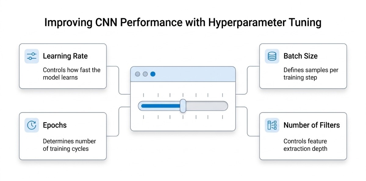
Once you have a working CNN model, the next step is improving its performance. This is where hyperparameter tuning becomes critical. Hyperparameters are the settings you define before training begins, and they directly influence how well your model learns, how fast it converges, and how accurately it generalizes to new data.
Instead of changing the architecture, tuning these values allows you to optimize results without increasing unnecessary complexity.
Learning Rate
The learning rate determines how much the model updates its weights after each iteration, which means controlling how fast the model learns. If the learning rate is too high, the model may skip optimal solutions and fail to converge. If it is too low, training becomes very slow and may get stuck in local minima.
A well-balanced learning rate ensures that the model learns efficiently while maintaining stability during training. In practice, starting with a moderate value (like 0.001 for Adam optimizer) and adjusting based on performance is a common approach.
Learning rate schedulers or decay strategies can further improve results by reducing the rate as training progresses.
Batch Size
Batch size defines how many samples are processed before updating the model weights. Smaller batch sizes lead to more frequent updates, which can improve generalization but may introduce noise in learning.
Larger batch sizes provide more stable gradients and faster computation, but may require more memory and risk poorer generalization.
Choosing the right batch size is a trade-off between training speed, memory usage, and model performance. For most CNN tasks, values like 32 or 64 provide a good balance.
Epochs
An epoch represents one complete pass through the entire training dataset. Training for too few epochs results in underfitting, where the model fails to learn meaningful patterns.
Training for too many epochs can lead to overfitting, where the model memorizes the training data instead of generalizing.
The key is to monitor performance over time and stop training when validation accuracy stops improving. Techniques like early stopping are often used to automatically determine the optimal number of epochs.
Number of Filters
The number of filters in convolution layers determines how many features the model can learn at each stage. Fewer filters may limit the model’s ability to capture complex patterns, while too many filters increase computational cost and risk overfitting.
Typically, CNNs start with a smaller number of filters (like 32) in early layers and increase them in deeper layers (64, 128, etc.)
This allows the model to gradually learn more complex features while maintaining efficiency.
Why This Matters
Each of these hyperparameters interacts with the others, and small changes can significantly impact performance. There is no one size fits all configuration, which is why tuning is often an iterative process based on experimentation.
By carefully adjusting learning rate, batch size, epochs, and filters, you can improve accuracy, reduce training time, and build a model that performs reliably on real world data.
How to Prevent Overfitting in CNN Models
Overfitting is one of the most common challenges when training Convolutional Neural Networks. It occurs when a model learns the training data too well, capturing noise and specific patterns instead of general features. As a result, the model performs very well on training data but fails to deliver accurate results on new, unseen data.
In real scenarios, this is a critical issue because the goal of any model is not just to memorize data but to generalize effectively. To address this, several practical techniques are used to improve generalization and make the model more robust.
Dropout
Dropout helps in reducing model dependency. It is a regularization technique where a fraction of neurons is randomly “dropped” during training. This means that at each iteration, certain neurons are ignored, forcing the network to learn more distributed and independent representations.
By preventing the model from relying too heavily on specific neurons, dropout reduces overfitting and improves the model’s ability to generalize. It is commonly applied in fully connected layers, with typical dropout rates ranging from 0.3 to 0.5.
Data Augmentation
Data augmentation artificially increases the size and diversity of the training dataset by applying transformations such as rotation, flipping, zooming, and shifting. This helps the model learn from varied versions of the same data, making it less sensitive to specific patterns.
Instead of collecting more data, augmentation creates new training examples, allowing the model to generalize better across different scenarios. This is especially useful when working with limited datasets.
Early Stopping
Early stopping monitors the model’s performance on validation data during training and stops the process when performance stops improving. This prevents the model from continuing to learn noise and overfitting the training data.
By halting training at the right time, early stopping ensures that the model retains its ability to generalize while avoiding unnecessary computation.
Techniques like dropout, data augmentation, and early stopping work together to improve generalization, stabilize training, and ensure that the model learns meaningful patterns rather than memorizing data.
Transfer Learning with Pretrained CNN Models
As CNN models become deeper and more powerful, training them from scratch is often unnecessary and inefficient, especially when you have limited data. This is where transfer learning becomes highly valuable. Instead of building a model from the ground up, you start with a pretrained network that has already learned rich visual features and adapt it to your specific task.
What is Transfer Learning
Transfer learning is the process of reusing a model that has already been trained on a large dataset and applying it to a new but related problem. Most commonly, these models are trained on the ImageNet dataset, which contains over 1.2 million images across 1000 different classes.
During this training, the model learns fundamental visual features such as edges, textures, shapes, and object structures.
These learned features are not limited to one specific task. Instead, they act as a general visual understanding that can be transferred to other problems. This is why transfer learning works so effectively; it allows you to reuse knowledge instead of relearning everything from scratch.
In practical terms, this leads to faster training, better accuracy, and significantly reduced data requirements. Even with a relatively small dataset, a pretrained model can deliver strong performance because it already understands how to interpret visual patterns.
Using Pretrained Models for Custom Tasks
When applying transfer learning, a pretrained model such as VGG16 is typically used as a base. The earlier layers of the model, which capture general features like edges and textures, are retained. These layers do not need to be retrained because they already contain useful information.
The later layers are task-specific. These are either replaced or modified to match your problem, such as changing the number of output classes. New layers are added on top of the pretrained base to learn patterns specific to your dataset.
This approach allows the model to combine general visual knowledge with task-specific learning, resulting in a more efficient and accurate system. Instead of building everything from scratch, you are effectively refining an already intelligent model.
Feature Extraction vs Fine-Tuning
A key decision in transfer learning is whether to use the pretrained model as a fixed feature extractor or to fine-tune it further. This decision depends largely on the size and nature of your dataset.
When working with a small dataset, it is generally better to keep the pretrained layers frozen and use the model only for feature extraction. This prevents overfitting and ensures that the model relies on stable, well-learned features.
As the dataset size increases, you can begin to fine-tune the model by unfreezing some of the higher layers. This allows the model to adapt more deeply to your specific problem while still benefiting from the pretrained knowledge.
For very large datasets, deeper fine-tuning parameters can be applied to achieve even better performance. Understanding this balance is important because it helps you avoid unnecessary complexity while still maximizing model performance.
Popular Pretrained CNN Models
Modern deep learning frameworks like Keras provide access to several well-established pretrained CNN architectures, each designed with different trade-offs between accuracy and efficiency.
VGG models are known for their simplicity and structured design, making them easy to understand and widely used for transfer learning tasks.
ResNet introduced residual connections, enabling very deep networks to train effectively without performance degradation.
EfficientNet focuses on optimizing both accuracy and computational efficiency, making it suitable for scalable applications.
MobileNet, on the other hand, is designed for lightweight environments such as mobile and edge devices, where computational resources are limited.
Choosing the right model depends on your specific requirements, including dataset size, available hardware, and performance expectations.
Why Transfer Learning is the Standard Approach
In real-world applications, training a CNN from scratch is rarely the most practical option. Transfer learning provides a more efficient and effective alternative by leveraging pretrained models that already understand visual data at a fundamental level.
By reusing and adapting these models, you can build high-performing systems with less data, reduced training time, and improved accuracy.
This is why transfer learning has become the default approach in modern computer vision projects, from image classification to more advanced tasks like object detection and segmentation.
Real World Applications of Convolutional Neural Networks
Convolutional Neural Networks are not just theoretical models; they are widely used in real-world systems that rely on visual understanding. Their ability to automatically extract and interpret patterns from images makes them a core technology across multiple industries, and their adoption continues to grow rapidly with advancements in AI solutions.
In fact, the global deep learning image recognition market was valued at around $65 billion in 2025 and is projected to reach $250 billion by 2033, showing how central CNN-based systems have become in modern applications.
Image Recognition and Classification
One of the most common applications of CNNs is image recognition, where the model identifies and classifies objects within an image. This is used in technologies such as photo organization, visual search, and content moderation.
CNN-based image recognition systems have become the foundation of modern computer vision, replacing traditional methods due to their ability to automatically learn features and scale across millions of images.
Medical Imaging and Diagnosis
In healthcare, CNNs are transforming how medical images are analyzed. They are used to process X-rays, MRIs, and CT scans to detect diseases, identify abnormalities, and assist doctors in diagnosis.
Alongside image-based AI, technologies like natural language processing are also enhancing healthcare systems by enabling better analysis of clinical data and reports. Together, these advancements are making healthcare more data-driven and efficient.
Recent advancements show that CNNs are now considered state of the art for medical image analysis, enabling improvements in areas such as tumor detection, organ segmentation, and early disease diagnosis.
Self-Driving Cars and Autonomous Systems
CNNs play a critical role in self-driving cars by enabling real-time visual understanding. They are used to detect lanes, recognize traffic signs, identify pedestrians, and track surrounding vehicles.
These systems rely heavily on CNN-based perception models, which allow vehicles to interpret complex environments and make safe driving decisions. CNNs have become a foundational component in autonomous driving systems.
Face Detection and Recognition
CNN are widely used in face detection and recognition systems. They power features such as smartphone face unlock, security surveillance, and identity verification systems.
With the growing demand for bio metric authentication and security, CNN-based facial recognition continues to expand across industries, from consumer devices to large-scale surveillance systems.
From healthcare and transportation to security and consumer applications, CNNs enable systems to understand and act on visual data with high accuracy.
Their widespread adoption across industries and the rapid growth of the image recognition market clearly show that CNNs are not just important but foundational to modern AI systems.
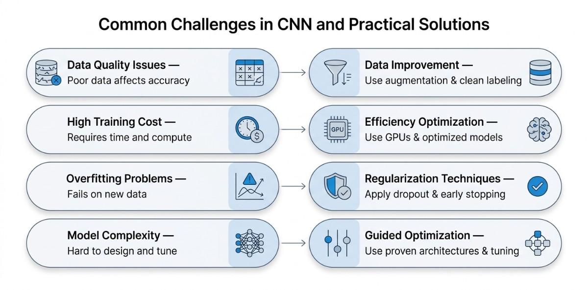
Common Challenges in CNN and Practical Solutions
Working with Convolutional Neural Networks is powerful, but it comes with practical challenges that can directly impact model performance, training efficiency, and real-world usability. Understanding these challenges early helps in building more reliable and scalable models.
Data Quality and Availability Issues
CNNs are highly dependent on large amounts of high-quality labeled data. If the dataset is too small, imbalanced, or contains noisy labels, the model struggles to learn meaningful patterns and often produces inaccurate predictions. Poor data quality directly affects generalization, making the model unreliable on new inputs.
To address this, improving data quality becomes essential. Techniques such as data augmentation can artificially expand the dataset by creating variations of existing images, while proper data cleaning ensures accurate labels.
Using pretrained models through transfer learning also helps reduce dependency on large datasets.
High Training Time and Computational Cost
Training CNNs, especially deeper architectures, can be computationally expensive and time-consuming. Large datasets combined with complex models can lead to long training cycles, slowing down experimentation and development.
This can be managed by using GPUs or cloud-based environments to speed up computation. Additionally, reducing model size, using optimized architectures like MobileNet or EfficientNet, and applying techniques such as batch normalization can improve training efficiency without sacrificing performance.
Overfitting and Poor Generalization
CNNs can easily overfit the training data, especially when the dataset is limited or the model is too complex. This results in high training accuracy but poor performance on unseen data, making the model ineffective in real-world scenarios.
To prevent overfitting, techniques like dropout, data augmentation, and early stopping are commonly used. Regularization methods and careful monitoring of validation performance also help ensure that the model learns general patterns instead of memorizing data.
Model Complexity and Optimization Challenges
Designing an effective CNN architecture can be challenging due to the large number of choices involved, such as the number of layers, filters, and hyperparameters. An overly complex model can increase computational cost and risk of overfitting, while a simpler model may fail to capture important features.
A practical approach is to start with proven architectures and gradually refine them based on performance. Hyperparameter tuning, using pretrained models, and experimenting with different configurations help in finding the right balance between accuracy and efficiency.
Final Thoughts
Convolutional Neural Networks have become the foundation of modern computer vision because they are specifically designed to understand visual data in a structured and efficient way. From learning basic features to making complex predictions, CNNs provide a complete framework for solving image-based problems.
The key takeaway is simple; use CNNs when your data has spatial structure, such as images or videos, and focus on building a strong pipeline that includes proper preprocessing, a well-designed model, and performance optimization.
Instead of aiming for complexity, prioritize clarity, data quality, and the right techniques like transfer learning and tuning to achieve reliable and scalable results.
 WhatsApp
 Call Us
 Mail Us